|
|
Inverse Dynamics |
[FrontPage Include Component] |
|
|
|
|
|
|||||
|
NAVIGATOR: Back - Home > Adi > Services > Support > Tutorials > Gait > Chapter2 : |
|||||
|
|
|||||
| |||||||||||||||||||
|
Inverse Dynamics
Categories
|
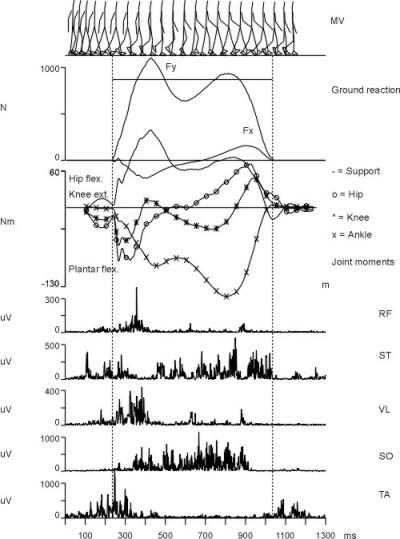
2.3 Principles of Gait DynamicsDynamics refer to accelerations and thereby forces. The movements during walking are generated by muscle forces, which act on the skeletal bones through lever arms thereby generating moments (or torque). This implies that an analysis of gait dynamics involves the calculation of net joint moments by inverse dynamics. Figure 2.3.1 illustrates a complete dynamical gait analysis in two dimensions.
Figure 2.3.1 The figure shows data from a single stride of one subject. On top a stick diagram illustrates the walking movements (every 4th frame is depicted). Below the stickdiagram the vertical (Fy) and horizontal (Fx) ground reaction force are drawn with a horizontal line indicating the body weight. A negative Fx indicates a braking force. The second Y-axis from the top shows the net joint moments about the ankle (x), knee (*) and hip joint (o). A total support moment for the whole leg is also shown as the unmarked line. The meaning of the moments will be explained below. Finally, the rectified EMG of m. rectus femoris, m. semitendinosus, m. vastus lateralis, m. soleus and m. tibialis anterior are shown in mV. It is shown on figure 2.3.1 that a negative moment about the ankle joint indicates dominance of the plantar flexor muscles, a positive knee joint moment extensor dominance and a positive hip joint moment flexor dominance. The reason for the signs of these moments can be understood from the following figure:
Figure 2.3.2 It is seen that the equation expressing the joint moment (Mj) consists of maximally 6 terms. Note that the terms s4* and s5* are only used for the foot and only during ground contact. For the leg and the thigh these two terms are always replaced by the terms s4 and s5. Procedure of calculation.This method is also called "The Free Body Segment Method", because we perform the calculations on one segment at a time assuming that the segment rotates about a transversal axis through the segment center of mass. To compute the net joint moment about the ankle joint we start with the foot segment during ground contact:
During the swing phase the ground reaction forces are none existent and no distal forces act on the foot segment, i.e. only terms s1, s2 and s3 go into the moment equation. When computing the net joint moment about the knee joint, the joint reaction forces Fxj and Fyj from the ankle joint are transfered to Fxd and Fyd acting on the distal end of the shank. They are then used in the terms s4 and s5 in the moment calculation. The term s6 consists only of the moment from the ankle joint. The methods assures that segmental interaction is accounted for and part of the calculation. Note that the joint reaction forces only are used once when calculating the ankle joint moment. However, the ground reaction forces "travel" to the shank and the thigh through the transferred joint reaction forces, which are added in the calculation of the new proximal joint reaction forces. The hip joint moment is calculated exactly the same way as the knee joint moment. Muscle dominance.The approach illustrated in figure 2.3.1. requires the subject to move from left to right. If the direction of movement was changed from right to left the joint moments would change polarity. The convention used here is that a joint moment pulling in a counterclockwise direction is positive. The pulling direction refers to the force of the dominating muscle group. However, the pulling direction does not indicate the direction of movement, i.e. flexion or extension at the actual joint. If we consider a situation where the net joint moment about the knee joint is positive and the joint angular velocity negative, we have a situation with a knee joint extensor moment while at the same time the joint is flexing. This means that the knee joint extensor muscles (m. quadriceps femoris) contract eccentrically, i.e. the active muscle fibers are being stretched by an external moment larger than the muscle moment acting about the joint. Therefore, inspection of the joint movement provides information about concentric or eccentric muscle contractions. Multiplication of joint moment and joint angular velocity can provide joint power (see later). The polarity of the net joint moment alone indicates the dominating muscle group. In the case of a two-dimensional approach the muscle groups in question will always be extensors or flexors (at the ankle joint dorsi or plantar flexors). The term "dominance" is used because a net joint moment of a certain value (in Newton x meter) may be the result of both extensors and flexors acting about the joint simultaneously. This situation is called "co-contraction" and the only way we can know whether co-contraction takes place or not is to record EMG at the same time (see figure 2.3.1). It follows that a net joint moment of zero Nm may be generated by "maximal" co-contraction or no muscle activity at all, because the calculated moment represent the "net" result of all muscles acting about the joint. Figure 2.3.3 below shows a typical ankle joint moment from the stance phase of normal walking at 4.5 km/h. It is seen that the net joint moment is negative during the entire stance phase. This means that the moment is generated by the plantar flexors, i.e. mainly the soleus and the gastrocnemius muscles. The moment is expressed relative to the body mass, which allows to compare different joint moments to each other and also across subjects.
Figure 2.3.3. Ankle joint moment from one subject. Figure 2.3.4. shows a typical net knee joint moment from a normal subject walking at 4.5 km/h. As for the previous figure only the stance phase is shown and the moment is normalized to body mass. At heel strike and shortly after the moment is flexor dominated, which is believed to reduce horizontal velocity at impact. Then a relatively large peak extensor moment is seen. During this period the knee joint is first being flexed and then extended. This implies that we have an eccentric contraction of m. quadriceps femoris followed by a concentric contraction of the same muscle. In the middle of stance the moment drops towards zero and in many subjects it goes negative, i.e. flexor dominance (see e.g. figure 2.3.1). At the end of the stance phase the moment turns back to extensor dominance, but normally showing a much lower peak value than the first extensor peak. The muscles responsible for the last extensor peak is still unknown, however occasionally the m. rectus femoris is active during this period. The contraction is, however, eccentric since the knee joint is being flexed.
Figure 2.3.4. Knee joint moment from one subject Figure 2.3.5. below shows a typical hip joint moment from a normal subject walking at 4.5 km/h. Only the stance phase is shown and the moment is normalized to body mass. The hip joint moment is normally extensor dominated during the first half or 2/3 of the stance phase and flexor dominated in the remaining period. The extensor moment is generated by the hamstring muscles and the flexor moment is believed to be produced by m. iliopsoas. However, this muscles is so difficult to record EMG from that the flexor moment still can be termed "unexplained"
Figure 2.3.5. Hip joint moment from one subject Conventions of polarity.We have here described a typical two-dimensional analysis of gait dynamics. In the literature it has been most common to use the formulas shown here with a positive moment pulling in a counterclockwise direction. However, some authors prefer to consider all extensor moments positive. It is therefore good practice to indicate a zero-line on all figures and some labels indicating the meaning of polarity. Often a so-called "total support moment" is calculated by adding up the ankle, knee and hip joint moment (see figure 2.3.1). To give this parameter a physiological meaning it is, however, necessary to consider extensor moments positive. The support moment is said to represent the total action of the whole leg to 1) generate the walking velocity and 2) prevent the leg from collapsing. Note that three-dimensional inverse dynamics often calculates net joint moments with a polarity opposite to the 2D-approach shown here. This does not mean that the 3D-moments are wrong. Warning.A simplified approach to calculate joint moments is often seen. These moments are termed "external joint moments" and they do not include inertial moments, linear accelerations or segment interaction. Often the polarity of an external moment may be opposite to the "real moment" calculated by inverse dynamics. Accordingly the method is considered inferior and too simplified. |
|
|