APASview

Introduction

The ARIEL APASVIEW software module has been developed for dynamically viewing stick figures, numerical data and AVI videos. The APASview software module makes it possible to load all data into the computer and simultaneously display and evaluate multiple data sets for a desired sequence.
Although a few of the APASView's features may appear complex, they are relatively easy to master once you understand the underlying concepts. This manual is arranged to teach you these concepts in a logical order by showing you, in step-by-step fashion, how to use APASView.

TO START THE APASVIEW PROGRAM:

1. Double-click the APASVIEW icon located in the APAS System window group. The main APASVIEW window will appear. The APASView VCR Control panel will be displayed in the center of the screen.

SCREEN LAYOUT:

Prior to creating an APASView project, you should take the time to familiarize yourself with the format and contents of the various screens listed below:

THE APASView VCR CONTROL MENU:

The APASView VCR Control menu is designed to mimic the controls on a typical VCR. Besides the normal buttons for controlling a sequence (Play, Stop, Pause, Step Forward, Step Reverse and Single/Continuous Play) the VCR Control menu also includes options for synchronization, display speed and zooming.

Frame - Shows the frame number currently being displayed. It is possible to edit this value to "jump" to a particular frame.
Step - This parameter is used to skip frames in the sequence. If this value is 1, every frame/numerical value is displayed. If the value is 2, only every second frame/numerical value is displayed. This parameter is quite useful if the sequence contains a lot of data sampled at a high rate.

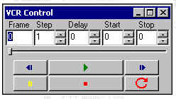
Delay - This parameter is used to control the speed of the animation in the "play" mode. Larger numbers represent longer delays between successive images.

Start - This parameter is used in combination with the Stop parameter to "zoom" the sequence. The Start value is used to specify the first frame/numerical value that will be displayed in a sequence. All active windows will use the Start value.
Stop - This parameter is used in combination with the Start parameter. Stop indicates the last frame/numerical value that will be displayed in a sequence.
SETTING START AND STOP PARAMETERS USING THE DATA WINDOW

Click and hold the right mouse button in the Data Windows, move the mouse left or right. This will mark a specific area of interest in the data signal with dashed vertical lines. Release the mouse button to select the area and the Start and Stop parameters will automatically be adjusted.

THE MAIN APASView TOOL BAR:

The tool bar is located near the top of the window. Icons are pictorial representations of commands or functions. You can access the following commands by clicking the appropriate icon.

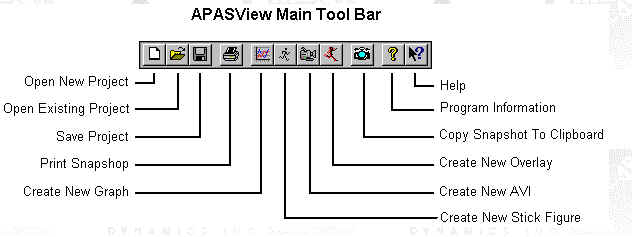
Open New Project - Selected to create a new APASView project file.
Open Existing Project - Selected to open a previously created APASView project file.
Save Project - Selected to save the current active windows to an APASView project.
Print Snapshot - Selected to print a snapshot of the current application.
Create New Graph - Selected to create a new graph window.
Create New Stick Figure - Selected to create a new stick figure window.

Create New AVI - Selected to create a new AVI window.
Create New Overlay - Selected to create a new overlay window.
Copy - Selected to copy the snapshot to the Windows clipboard.
About - Selected to display program information.
Help - Selected to display the APASView help information.

DATA WINDOW DISPLAY:

he Data Window can be used to display almost any kind of numerical data collected over time. For example, displacement, velocity, acceleration, segment angles joint angles, force, EMG and more.
Producing a graph is a two-step process. First, individual data curves are specified and the data values are read and saved in the display grid. Second, the actual graph is drawn, using these data curves.

THE GRAPH WINDOW TOOL BAR:

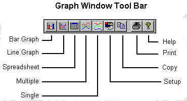
Bar Graph - Changes specified data to bar graph format
Line Graph - Changes specified data to line graph format
Spreadsheet - Changes specified data to spreadsheet format
Multiple - Displays all the specified data on a single graph
Single - Displays each data curve on an individual line graph
Setup - Selected to modify/edit the contents of the Graph window.
Copy - Copies the current contents to the Windows clipboard

Print - Prints the current contents to the printer
Help - Displays the help topics for the Graph Window

CREATING A NEW GRAPH WINDOW:

he basic steps for creating a Graph window are listed below.

1. Select DISPLAY, NEW DATA (or the NEW GRAPH icon in the main Toolbar) to open the Data ViewSetup menu.

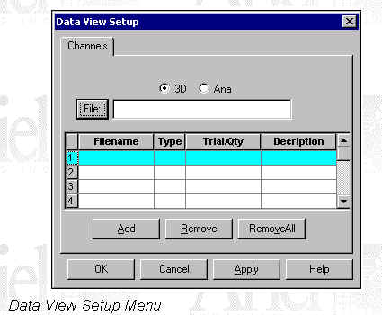
2. Specify the desired data as either 3D (video data) or ANA (analog data).
3. Click the FILE button and double-click the desired APAS data file. This file is created by the Transform module and has a *.3D extension.
4. Click the ADD button to open the Specify 3D Data Trial menu.

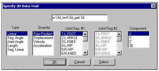
5. Select the desired Type (Linear, Segment Angle, Joint Angle, Length and Segment Linear), Quantity, Joint/Seg(s) and Component. Clicking the SELECT button will add the current selections to the data table and leave the menu open for additional selections while clicking the OK button will add the current selections and close the menu.

6. Click the OK button on the Data View Setup menu to graph the selected data.
7. Select the desired display options from the Graph Windows Toolbar. Available choices include Bar Graph, Line Graph, Spreadsheet and Single/Multiple Graph.
8. Select the PLAY button from the VCR control menu to animate the current selections.
9. The user may now save, analyze, and/or print the project.

LINEAR GRAPH:

Linear is selected to plot joint motion (displacement, velocity or acceleration) in the standard Cartesian coordinate system. An additional curve measure, Raw Position, may be selected for linear type curves. This measure represents the actual digitized position values prior to data smoothing. In the Cartesian system, motion is represented either by X, Y & Z coordinate components which are signed values with implicit direction, or by resultant "3D" magnitude which is an unsigned valued with no implicit direction. The coordinate system is the one selected for the "control points" used to calibrate the image space, and the units of measurement are those initially specified for this sequence.

The following steps are recommended for creating Linear plots.

1. Set the TYPE column to LINEAR.
2. Set the QUANTITY column to the desired parameter. Available choices are Raw Position, Displacement, Velocity and Acceleration.
3. Set the JOINT/SEGMENT #1 column to the desired joint. Available choices are determined by the Point ID's that were established in the Digitizing module.
4. Set the COMPONENT column to the desired parameter. Available choices are X, Y, Z and 3D (Magnitude).

5. Click the OK or SELECT button. NOTE: Clicking the SELECT button will add the selected data set(s) to the list of data sets in the grid without leaving the dialog box. This allows additional entries to be made to the grid. Select the OK button to enter the selected data set to the active data set display and close the current menu.
6. Select the OK button on the Data View Setup menu to display the graph in a new window.

7. Use the icons on the Graph Window tool bar to display the data in the desired format.

SEGMENT ANGLE GRAPH:

The digitized figure can be described as segments linked together at the joints and is basically a system of moving segments or links. Segment Angle is selected to plot the motion (displacement, velocity or acceleration) of an individual SEGMENT about one endpoint in the polar coordinate system. In this system, motion is represented by an angular component about the pole (segment endpoint) as viewed along one of the coordinate axis directions. Angular units are always the same (degrees) regardless of the linear units chosen for this sequence. Segment angles are selected from the list of segments for a project as determined by the joint connection table.

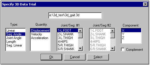
The following steps are recommended for creating Segment Angle plots.

1. Set the TYPE column to SEG ANGLE.
2. Set the QUANTITY column to the desired parameter. Available choices are Displacement, Velocity and Acceleration.
3. Set the JOINT/SEGMENT #1 column to the desired segment. Available choices are determined by the segments that were established in the Digitizing module.
4. Set the COMPONENT column to the desired parameter. Available choices are X, Y, and Z. For segment angle curves, this component represents the viewing axis. (Selecting Z would display the angle projection on the X-Y plane.)

5. Select the COMPLEMENT option to display the complement angle.
6. Click the OK or SELECT button. NOTE: Clicking the SELECT button will add the selected data set(s) to the list of data sets in the grid without leaving the dialog box. This allows additional entries to be made to the grid. Select the OK button to enter the selected data set to the active data set display and close the current menu.
7. Select the OK button on the Data View Setup menu to display the graph in a new window.

8. Use the icons on the Graph Window tool bar to display the data in the desired format.

JOINT ANGLE GRAPH:

Joint Angle is usually selected to plot the motion (displacement, velocity or acceleration) of one segment relative to another about the joint that they share in common. Motion is reported in the polar coordinate system as a relative angular component about the pole (joint) either as viewed along one of the coordinate axis direction, or as viewed along the perpendicular to the plane of the two segments. Angular units are always the same (degrees) regardless of the linear units chosen for this sequence. Joint angles are specified by selecting 2 segments from the segment list. In this way the angle between ANY two segments, not necessarily ones with a common joint, can be graphed.

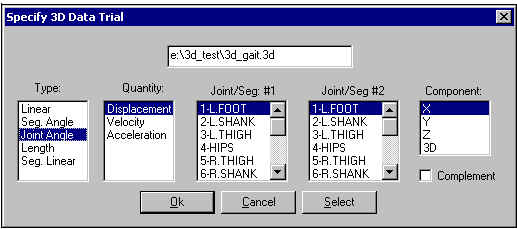
The following steps are recommended for creating Joint Angle plots.

1. Set the TYPE column to JOINT ANGLE.
2. Set the QUANTITY column to the desired parameter. Available choices are Displacement, Velocity and Acceleration.
3. Set the JOINT/SEGMENT #1 column to the first desired segment. Available choices are determined by the segments that were established in the Digitizing module.
4. Set the JOINT/SEGMENT #2 column to the second desired segment. Available choices are determined by the segments that were established in the Digitizing module.

5. Set the COMPONENT column to the desired parameter. Available choices are X, Y, Z and 3D.
6. Select the COMPLEMENT option to display the complement angle.
7. Select the OK button on the Data View Setup menu to display the graph in a new window.
8. Use the icons on the Graph Window tool bar to display the data in the desired format.

LENGTH GRAPH:

Length is selected to plot the linear distance between two joints. The units of measurement are those initially specified for this sequence. Lengths are specified by selecting 2 joints from the joint list. In this manner, the length between ANY two joints, not necessarily ones with a common segment, can be measured and graphed.

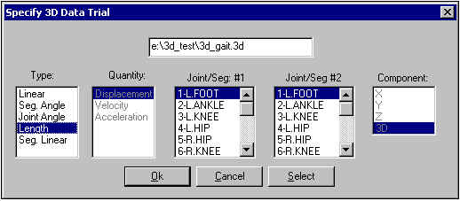
The following steps are recommended for creating Length plots.

1. Set the TYPE column to LENGTH.
2. Set the JOINT/SEGMENT #1 column to the first desired joint. Available choices are determined by the Point ID's that were established in the Digitizing module.
3. Set the JOINT/SEGMENT #2 column to the second desired joint. Available choices are determined by the Point ID's that were established in the Digitizing module.
4. Click the OK or SELECT button. NOTE: Clicking the SELECT button will add the selected data set(s) to the list of data sets in the grid without leaving the dialog box. This allows additional entries to be made to the grid. Select the OK button to enter the selected data set to the active data set display and close the current menu.

5. Select the OK button on the Data View Setup menu to display the graph in a new window.
6. Use the icons on the Graph Window tool bar to display the data in the desired format.

SEGMENT LINEAR GRAPH:

Segment Linear is selected to plot the "linear" components of a segment. The difference between Linear and Segment Linear is that the segment has a mass and a joint does not. When the Segment Linear option is specified, three new items are listed in the Qty column. Linear quantities of Force, Energy and Power are of a point concentrated at the segmental center-of-mass with a mass equal to the segment mass. The units of measurement are those initially specified for this sequence. 

The quantities are defined as: Force = Mass x Acceleration (Nt or Lbs) Energy = 0.5 x Mass x Velocity x Velocity (Nt-m or Ft-Lbs) Power = Force x Velocity (Nt-m/s or Ft-Lb/s)

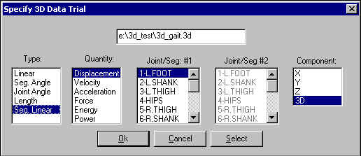
The following steps are recommended for creating Segment Linear plots.

1. Set the TYPE column to SEGMENT LINEAR.
2. Set the QUANTITY column to the desired parameter. Available choices are Displacement, Velocity, Acceleration, Force, Energy and Power.
3. Set the JOINT/SEGMENT #1 column to the desired segment. Available choices are determined by the Point ID's that were established in the Digitizing module.
4. Set the COMPONENT column to the desired parameter. Available choices are X, Y, Z and 3D (Magnitude). Note: Energy and Power are scalar quantities and have only a single 3D value.

5. Click the OK or SELECT button. NOTE: Clicking the SELECT button will add the selected data set(s) to the list of data sets in the grid without leaving the dialog box. This allows additional entries to be made to the grid. Select the OK button to enter the selected data set to the active data set display and close the current menu.
6. Select the OK button on the Data View Setup menu to display the graph in a new window.

7. Use the icons on the Graph Window tool bar to display the data in the desired format.

MODIFYING AN EXISTING GRAPH WINDOW:

The specified data in a Graph Window can be easily modified using the steps listed below.

1. Select the Setup icon from the Graph Window tool bar. This will display the Data View Setup menu and the currently specified data.
2. Make the desired changes by adding or removing data sets. Select the Remove or Remove All button with the desired data highlighted to delete current data sets. The Add button can be selected to add additional data curves.
3. Select the OK button from the Data View Setup menu to display the updated Graph Window.

GRAPHING OPTIONS:

The data in the Graph window can be displayed in several different formats including bar graphs, line graphs, spreadsheets and single or multiple axis graphs. The graph window options are generally specified by left-clicking the icons located in the Graph Window tool bar.
SELECTING A DATA INTERVAL
An additional option is provided by using the right mouse button. When performing an analysis, it may be helpful to limit the animation to a small portion of the displayed data curve. This can be accomplished using the steps listed below.

1. Position the cursor at the start of the area of interest on the data curve window.
2. Use the right mouse button to click and hold while dragging the cursor to the desired endpoint on the data curve. The start and end points will be designated by a dashed vertical line.
3. Releasing the mouse button will select the specified area and automatically update the Frame, Start and Stop times in the VCR Control menu.
4. Animating the sequence using the VCR Control buttons will limit the display to the currently selected area.

5. The display can be reset to the full original range by selecting the RESET RANGE command from the VIEW menu.

STICK WINDOW DISPLAY:

he Stick Window is designed for displaying marker trajectories as stick figures using APAS .3D files as the data source. Stick figures are created by connecting the body joint locations, or external segments like a golf club or tennis racket, with line segments according to the body connection information supplied when the sequence was created (digitizing process).
The stick figures by be displayed in single frame, multiple frame or animation mode. The size location and orientation of the stick figure can be set in any manner desired.

THE STICK WINDOW TOOL BAR:

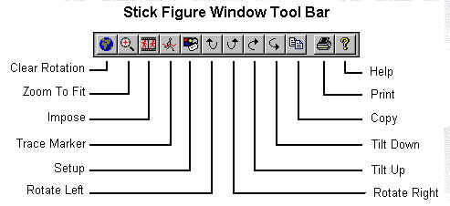
Clear Rotation - This icon is selected to rotate the stick figure to the original orientation (tilt angle = 0, pan angle = 0).
Zoom To Fit - This icon is selected to zoom the stick figure to fit the window size.
Impose - This icon is selected to impose the stick figure as a sequence.
Trace Marker - This icon is selected to toggle the "trace" function on/off for the specified marker(s).
Setup - This icon is selected to modify/edit an existing Stick Figure window.

Rotate Left - This icon is selected to rotate the stick figure 90 degrees to the left.
Rotate Right - This icon is selected to rotate the stick figure 90 degrees to the right.
Tilt Up - This icon is selected to rotate the stick figure 90 degrees up.
Tilt Down - This icon is selected to rotate the stick figure 90 degrees down.
Copy - Copies the current contents to the Windows clipboard
Print - Prints the current contents to the printer

Help - Displays the help topics for the Graph Window

CREATING A NEW STICK WINDOW:

The basic steps for creating a Stick Figure window are listed below.

1. Select DISPLAY, NEW STICK (or the NEW STICK3D icon in the main Toolbar) to open the Stick Figure View Setup menu.

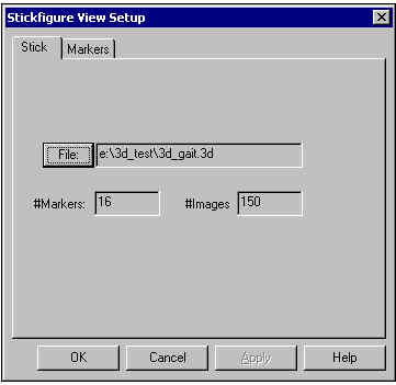
2. Click the FILE button and double-click the desired APAS data file. This file is created by the Transform module and has a *.3D extension. The path, number of markers and number of images will be displayed for the selected file.
3. Click the OK button on the Stick Figure View Setup menu to display the selected data.

4. Select the desired display options from the Stick Figure Windows Toolbar. Available choices include options for zooming, adding traces, imposing multiple stick figures, and rotating.
5. Select the PLAY button from the VCR control menu to animate the current selections.
6. The user may now save, analyze, and/or print the project.

MODIFYING AN EXISTING STICK FIGURE WINDOW:

The specified data in a Stick Figure Window can be easily modified using the steps listed below.

1. Select the Setup icon from the Stick Figure Window tool bar. This will display the Stick Figure View Setup menu and the currently specified data.
2. Make the desired changes by selecting the Stick or Markers tab.
3. Select the OK button from the Stick Figure View Setup menu to display the updated Stick Figure Window.

MARKER OPTIONS:

The APASView Video Window setup also allows the user to adjust the size and color of the joint markers and segments. This is often helpful for isolating a particular segment of the body for detailed analysis.

1. For a new Stick Figure Window, Select DISPLAY, NEW STICK (or the NEW STICK3D icon in the main Toolbar) to open the Stick Figure View Setup menu. For an existing Video Window, select the SETUP icon from the Stick Figure Window tool bar.

CHANGING MARKER PARAMETERS

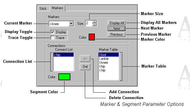
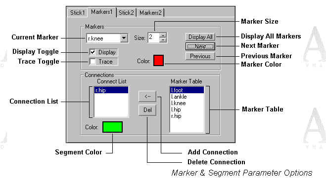
1. Select the Markers tab (if not already selected) to display the Marker parameters. The top half of the menu displays the marker information for the individual points.
2. Select the desired marker using the "down arrow" in the Current Marker field. A list of all the available markers will be displayed. A marker is selected by left-clicking the mouse on the desired label. The Next/Previous buttons can also be used to sequentially advance/reverse through the list of available markers. In the example shown above, the current point is the right knee (r.knee).

3. Select the desired marker Size using the up/down arrow keys or typing the desired size. A lower number represents a smaller marker larger numbers will display a larger marker. The acceptable size range is 0 to 5. The example above is set to the system default of 2.
4. Set the marker Color by left-clicking on the color button. This will display a palette of available color choices. The color for the current marker is selected by left-clicking on the desired color choice. In the example above, the right knee will be displayed in red. If the Trace option is activated for the current marker, the trace will also be displayed using this same color.

5. Set the Display Toggle to indicate whether the current marker will be displayed or not. A left-click of the mouse will add a check mark to the left of the Display label and will display the marker. Another left-click will remove the check mark and the current marker will not be displayed. In the example above, the Display option for the right knee is active, thus this marker will be displayed.
6. Set the Trace Toggle to indicate a trace will be displayed for the current marker or not. A left-click of the mouse will add a check mark to the left of the Trace label and will activate the trace function on the current marker using the marker color. Another left-click will remove the check mark and the trace on the current marker will not be displayed. The Trace function is toggled on/off from the main window tool bar. In the example above, the Trace option for the right knee is not active, thus there will not be a trace put on the display.

7. Select the Display All button to display all markers for the sequence.
8. Select the Next button to advance to the next marker in the available list. This list of markers is established in the Digitizing process when the points are originally defined. This will also add the current marker to the Marker Table in the Connection section on the lower half of the menu box.
9. Select the Previous button to back-up to the previous marker in the available list.

CHANGING SEGMENT PARAMETERS
The APASView program will automatically read the point connections that were originally established in the Digitizing process, however, the user has the option to modify these connections for the APASView project file.

1. Select the Markers tab (if not already selected) to display the Marker parameters. The bottom half of the menu displays the connection information for the individual points.
2. Select the connecting marker using the "down arrow" in the Current Marker field. A list of all the available markers will be displayed. A marker is selected by left-clicking the mouse on the desired label. The Next/Previous buttons can also be used to sequentially advance/reverse through the list of available markers. In the example shown above, the current point is the right knee (r.knee).

3. The Current Marker will be connected to all points listed in the Connection List. The Color of the segment connecting two points can be viewed and/or modified by clicking the desired point in the Connection List. The current color will be displayed in the segment Color box. Click the Color box to change the current color. In the example above, the Right Knee is connected to the Right Hip and the segment color is green.
4. Additional connected can be made by highlighting the desired point in the Marker Table and then selecting the Add Connection button. This will add the desired point to the Connection List. The color for the new segment can be viewed and/or modified using the steps listed above.

5. Point connections can be removed by highlighting the desired point in the Connection List and then selecting the Delete Connection button.
6. Select the OK button to display the changes. The CANCEL button is selected to abort the current menu without making any changes.

OVERLAY WINDOW DISPLAY:

The Overlay Window is designed for displaying two different stick figures in the same window. This is only possible using APAS .3D files as the data source. The Overlay Window is identical to the Stick Figure Window with the added option of simultaneously displaying two stick figures. After the data is loaded into the window the same features can be used in the Overlay Window.

THE OVERLAY WINDOW TOOL BAR:

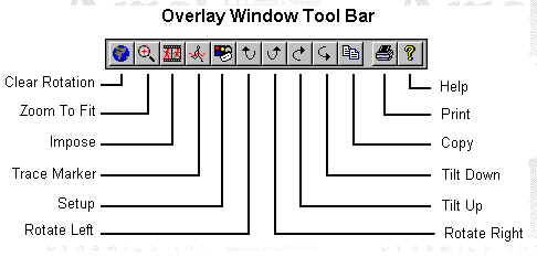
Clear Rotation - This icon is selected to rotate the stick figure to the original orientation (tilt angle = 0, pan angle = 0).
Zoom To Fit - This icon is selected to zoom the stick figure to fit the window size.
Impose - This icon is selected to impose the stick figure as a sequence.
Trace Marker - This icon is selected to toggle the "trace" function on/off for the specified marker(s).
Setup - This icon is selected to modify/edit an existing Stick Figure window.

Rotate Left - This icon is selected to rotate the stick figure 90 degrees to the left.
Rotate Right - This icon is selected to rotate the stick figure 90 degrees to the right.
Tilt Up - This icon is selected to rotate the stick figure 90 degrees up.
Tilt Down - This icon is selected to rotate the stick figure 90 degrees down.
Copy - Copies the current contents to the Windows clipboard
Print - Prints the current contents to the printer

Help - Displays the help topics for the Graph Window

CREATING A NEW OVERLAY WINDOW:

The basic steps for creating an Overlay window are listed below.

1. Select DISPLAY, NEW OVERLAY (or the NEW OVERLAY icon in the main Toolbar) to open the Overlay View Setup menu. Notice there are tabs available for Stick Figure/Markers #1 and Stick Figure/Markers #2.

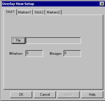
2. Select the Stick 1 tab, click the FILE button and then double-click the first desired APAS data file. This file is created by the Transform module and has a *.3D extension. The path, number of markers and number of images will be displayed for the selected file.

3. Select the Stick 2 tab, click the FILE button and then double-click the second desired APAS data file.
4. Click the OK button on the Stick Figure View Setup menu to display the selected data.
5. Select the desired display options from the Stick Figure Windows Toolbar. Available choices include options for zooming, adding traces, imposing multiple stick figures, and rotating.
6. Select the PLAY button from the VCR control menu to animate the current selections.

7. The user may now save, analyze, and/or print the project.

MARKER OPTIONS:

The APASView Video Window setup also allows the user to adjust the size and color of the joint markers and segments. This is often helpful for isolating a particular segment of the body for detailed analysis.

1. For a new Overlay Window, Select DISPLAY, NEW OVERLAY (or the NEW OVERLAY icon in the main Toolbar) to open the Overlay View Setup menu. For an existing Overlay Window, select the SETUP icon from the Overlay Window tool bar.

CHANGING MARKER PARAMETERS

1. Select the Markers 1 or 2 tab for the corresponding Stick Figure (if not already selected) to display the Marker parameters. The top half of the menu displays the marker information for the individual points.
2. Select the desired marker using the "down arrow" in the Current Marker field. A list of all the available markers will be displayed. A marker is selected by left-clicking the mouse on the desired label. The Next/Previous buttons can also be used to sequentially advance/reverse through the list of available markers. In the example shown above, the current point is the right knee (r.knee).

3. Select the desired marker Size using the up/down arrow keys or typing the desired size. A lower number represents a smaller marker larger numbers will display a larger marker. The acceptable size range is 0 to 5. The example above is set to the system default of 2.
4. Set the marker Color by left-clicking on the color button. This will display a palette of available color choices. The color for the current marker is selected by left-clicking on the desired color choice. In the example above, the right knee will be displayed in red. If the Trace option is activated for the current marker, the trace will also be displayed using this same color.

5. Set the Display Toggle to indicate whether the current marker will be displayed or not. A left-click of the mouse will add a check mark to the left of the Display label and will display the marker. Another left-click will remove the check mark and the current marker will not be displayed. In the example above, the Display option for the right knee is active, thus this marker will be displayed.
6. Set the Trace Toggle to indicate a trace will be displayed for the current marker or not. A left-click of the mouse will add a check mark to the left of the Trace label and will activate the trace function on the current marker using the marker color. Another left-click will remove the check mark and the trace on the current marker will not be displayed. The Trace function is toggled on/off from the main window tool bar. In the example above, the Trace option for the right knee is not active, thus there will not be a trace put on the display.

7. Select the Display All button to display all markers for the sequence.
8. Select the Next button to advance to the next marker in the available list. This list of markers is established in the Digitizing process when the points are originally defined. This will also add the current marker to the Marker Table in the Connection section on the lower half of the menu box.
9. Select the Previous button to back-up to the previous marker in the available list.

CHANGING SEGMENT PARAMETERS
The APASView program will automatically read the point connections that were originally established in the Digitizing process, however, the user has the option to modify these connections for the APASView project file.

1. Select the Markers tab (if not already selected) to display the Marker parameters. The bottom half of the menu displays the connection information for the individual points.
2. Select the connecting marker using the "down arrow" in the Current Marker field. A list of all the available markers will be displayed. A marker is selected by left-clicking the mouse on the desired label. The Next/Previous buttons can also be used to sequentially advance/reverse through the list of available markers. In the example shown above, the current point is the right knee (r.knee).

3. The Current Marker will be connected to all points listed in the Connection List. The Color of the segment connecting two points can be viewed and/or modified by clicking the desired point in the Connection List. The current color will be displayed in the segment Color box. Click the Color box to change the current color. In the example above, the Right Knee is connected to the Right Hip and the segment color is green.
4. Additional connected can be made by highlighting the desired point in the Marker Table and then selecting the Add Connection button. This will add the desired point to the Connection List. The color for the new segment can be viewed and/or modified using the steps listed above.

5. Point connections can be removed by highlighting the desired point in the Connection List and then selecting the Delete Connection button.
6. Select the OK button to display the changes. The CANCEL button is selected to abort the current menu without making any changes.

VIDEO WINDOW DISPLAY:

The Video Window is designed for displaying the video (AVI files) together with stick figures. This is an important feature since it allows the examiner to actually "see" where the data originated. Any questions in the data can be isolated to the exact image to observe what is actually happening.

THE AVI WINDOW TOOL BAR:

You can activate many functions by selecting the icons located on the VIDEO WINDOW tool bar.

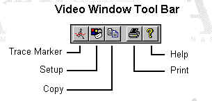
Trace Marker - This icon is selected to toggle the "trace" function on/off for the specified marker(s).
Setup - This icon is selected to modify/edit an existing Stick Figure window.
Copy - Copies the current contents to the Windows clipboard
Print - Prints the current contents to the printer

Help - Displays the help topics for the Graph Window

CREATING A NEW VIDEO WINDOW:

The basic steps for creating a Video window are listed below.

1. Select DISPLAY, NEW VIDEO (or the NEW STICK2D/AVI icon in the main Toolbar) to open the Stick Figure View Setup menu.
2. Select the AVI tab to display the video parameters.

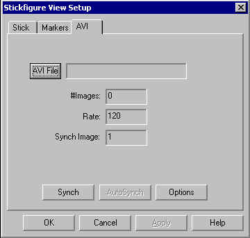
3. Click the AVI FILE button and locate the desired AVI file. Then double-click the AVI video file to display the video properties. This includes the file location, number of images, recording rate and synchronizing image number.
4. Click the SYNCH button to display the Select Synch Video Frame menu.

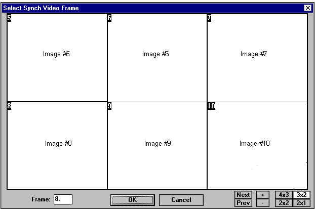
5. Click on the image used for synchronization. Images can be advanced/reversed one at a time using the +/- buttons. The Next/Previous buttons are used to advance a full panel of images. The size of the panel can be modified using the buttons in the lower right corner of the menu. Select the OK button to return to the AVI parameters menu. Select CANCEL to return without saving any changes.
6. Click the OPTIONS button to make certain the Field Order, Separate Frames and Speed settings are correct for the selected video file. Refer to the Video Options section for additional information. Select the OK button to save the changes and return to the AVI parameters menu. Select CANCEL to return without saving any changes. 

NOTE: This step is optional for the full version of APAS software as these settings should be specified during the trimming process in the TRIM module.

7. Select the OK button on the Stick Figure View Setup menu to display the AVI file in the video window.
8. Select the PLAY button from the VCR control menu to animate the current selections.
9. The user may now save, analyze, and/or print the project.

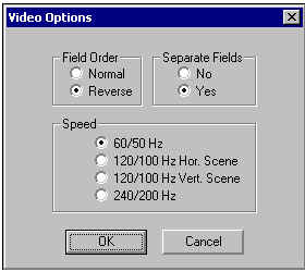
VIDEO OPTIONS:

FIELD ORDER

A standard video picture is made up of odd and even lines across the screen. Television standards require these lines to be interlaced. This means only half of the lines are displayed in one field. The first (odd) set of lines is displayed in the first field while the second (even) set of lines is displayed in the second field. These two fields comprise a frame, which is a complete picture.
Depending on the hardware and software combinations used for recording and displaying the AVI files, it is possible for the order of the displayed fields to be reversed. For this reason, the Ariel APASView program provides the option to specify the order for displaying the AVI files.

If it appears that the images are "jerky" or are being displayed in a "zigzag" manner, the field order probably needs to be reversed. The field order is specified using the following steps.

1. Select the OPTIONS menu to display the list of video options. Left-click either Normal or Reverse in the FIELD ORDER section. The current selection is indicated by the black dot to the left of the option. NOTE: When this option is changed, it affects all other APAS software modules where the AVI file can be displayed (Capture, Digitize, Display, Vectors etc.)
2. Select OK to proceed and save changes or CANCEL to abort.

SEPARATE FIELDS

Older models of the APAS capture an analog video signal using a step capture process and a computer controlled VCR. When using the "step capture" mode, the software and VCR work in conjunction to capture only the field information from the video signal. Therefore, when using video captured from the "step capture" process, the field information is already separated and this setting should be set to NO.
Capturing digital video in real-time results in the entire frame being captured. The field information is obtained by separating the frame into the two respective fields. This is required when using digital video files and is automatically set to YES.

SPEED

The APAS is capable of digitizing from any of various video formats. These formats can be determined by a variety of factors including the type of camera used for video recording, the make and model of frame grabber as well as the selected frame rate for recording. When using the JVC digital camcorder in the high-speed mode, video images are split to either one-half or one-quarter of the original size. The user must indicate which speed and/or JVC mode was used for the video recording to allow the software to correctly separate the images during the digitizing process.

1. 60/50 Hz - Select this option when using either NTSC/PAL video formats or Digital Video (DV) in the Normal Record mode.
2. 120/100 Hz Horizontal Scene - Select this option when using the JVC Digital Video camera in the 2X Horizontal High-Density mode. This mode is suitable for recording horizontally moving activities such as running.
3. 120/100 Hz Vertical Scene - Select this option when using the JVC Digital Video camera in the 2X Vertical High-Density mode. This mode is suitable for recording vertically moving activities such as golf.

4. 240/200 Hz - Select this option when using the JVC Digital Video camera in the 4X High-Density mode. This mode is suitable for recording fast moving activities.

MODIFYING AN EXISTING VIDEO WINDOW:

The specified data in a Video Window can be easily modified using the steps listed below.

1. Select the Setup icon from the Video Window tool bar. This will display the Stick Figure View Setup menu and the currently specified data.
2. Make the desired changes by selecting the Stick, Markers or AVI tab.
3. Select the OK button from the Stick Figure View Setup menu to display the updated Video Window.

APASVIEW PROJECT FILES:

he APASView program provides several different methods for saving the current project into a single file.

1. Select SAVE command from the FILE menu and specify the path and name for the current project file. The *.prj extension will automatically be added.OR
2. Select SAVE AS command from the FILE menu to save the current project with a new name. Specify the path and filename.OR
3. Click the SAVE icon located in the APASView tool bar.

OPENING A PROJECT FILE:

In order to open an existing APASView project file, use one of the following options.

1. Select OPEN command from the FILE menu and specify the path and file name of the desired project file.OR
2. Click the OPEN icon located in the APASView tool bar.

CREATING A NEW PROJECT FILE:

It is often desirable to create several different project files for a complete analysis. Each project could have a different configuration or illustrate a particular aspect of a study. A new project file is easily created for this purpose.

1. Select the NEW command from the FILE menu.OR
2. Select the NEW file icon from the APASView tool bar.

APASView QUICK REFERENCE:

GRAPH WINDOW

1. Select DISPLAY, NEW DATA (or the NEW GRAPH icon in the Toolbar) to open the Data View Setup menu.
2. Specify the desired data as either 3D (video data) or ANA (analog data).
3. Click the FILE button and double-click the desired APAS data file. This file is created by the Transform module and has a *.3D extension.
4. Click the ADD button to open the Specify 3D Data Trial menu.
5. Select the desired Type, Quantity, Joint/Seg(s) and Component. Clicking the SELECT button will add the current selections to the data table and leave the menu open for additional selections while clicking the OK button will add the current selections and close the menu.

6. Click the OK button on the Data View Setup menu to graph the selected data.
7. Select the desired display options from the Graph Windows Toolbar. Available choices include Bar Graph, Line Graph, Spreadsheet and Single/Multiple Graph.
8. Select the PLAY button from the VCR control menu to animate the current selections.
9. The user may now save, analyze, and/or print the project.

STICK FIGURE WINDOW

1. Select DISPLAY, NEW STICK (or the NEW STICK3D icon in the Toolbar) to open the Stick Figure View Setup menu.
2. Select the Stick tab.
3. Click the FILE button and double-click the desired APAS data file. This file is created by the Transform module and has a *.3D extension.
4. Select the Markers tab to modify the Marker parameters and Connection information. (This is optional).
5. Click the OK button on the Stick Figure View Setup menu to display the selected stick figure

6. Select the desired display options from the Graph Windows Toolbar. Available choices include Bar Graph, Line Graph, Spreadsheet and Single/Multiple Graph.
7. Select the PLAY button from the VCR control menu to animate the current selections.
8. The user may now save, analyze, and/or print the project.

OVERLAY WINDOW

1. Select DISPLAY, NEW OVERLAY (or the NEW OVERLAY icon in the Toolbar) to open the Stick Figure View Setup menu.
2. Select the Stick1 tab.
3. Click the FILE button and double-click the desired APAS data file. This file is created by the Transform module and has a *.3D extension.
4. Select the Markers1 tab to modify the Marker parameters and Connection information. (This is optional).
5. Repeat steps 2, 3 and 4 above for the second stick figure (Stick2 and Markers2).

6. Click the OK button on the Stick Figure View Setup menu to display the selected stick figure
7. Select the desired display options from the Graph Windows Toolbar. Available choices include Bar Graph, Line Graph, Spreadsheet and Single/Multiple Graph.
8. Select the PLAY button from the VCR control menu to animate the current selections.
The user may now save, analyze, and/or print the project.

VIDEO WINDOW

1. Select DISPLAY, NEW VIDEO (or the NEW STICK2D/AVI icon in the Toolbar) to open the Stick Figure View Setup menu.
2. Select the AVI tab
3. Click the AVI FILE button and locate the desired AVI file. Then double-click the AVI video file to display the video properties. This includes the file location, number of images, recording rate and synchronizing image number.
4. Click the SYNCH button to display the Select Synch Video Frame menu

5. Click on the image used for synchronization. Select the OK button to return to the AVI parameters menu. Select CANCEL to return without saving any changes.
6. Click the OPTIONS button to set the video parameters VIDEO OPTIONS. Select the OK button to save the changes and return to the AVI parameters menu. Select CANCEL to return without saving any changes
7. Select the Markers tab to modify the Marker parameters and Connection information. (This is optional).

8. Select the Stick tab to superimpose a stick figure on the video. (This is optional).

SAVING AN APAVIEW PROJECT

1. Select FILE, SAVE and specify the path and file name for the APASView project file. The *.prj extension will be added to the file.

APASVIEW MENUS:

New
Selected to create a New APASView project. A single project consists of one or more windows to display graphs, stick figures, video and/or tabular data.
Open
Selected to open an existing APASView project file.
Close
Selected to Close the current project file.
Save
Selected to Save the current project file.
SaveAs
Selected to Save the current project file using a different file name.
Print
Print the current file on the selected printer.
Print Preview

Selected to check or examine the positioning on one or more pages. When you give the Print Preview command, a new window will be open showing the document position as it would appear on paper. To close the Print Preview window, select the Cancel button to go to the previous mode.
Print Setup
Selected to adjust the printer settings prior to issuing the PRINT command.
Recent Files
Displays a list of the most recent files that have been used in the Transformation module.

APAS Modules
Selected to open additional APAS modules while keeping the current program open. When this command is selected, the user will be presented with a list of APAS modules.
Exit
Selected to EXIT the APASView program.

EDIT COMMAND MENU:

Undo
Select the Undo command to undo the last change and restore the item that was deleted, replaced or changed. This command restores the item to the way it was before the last edit.
Cut
Select the Cut command to remove the selected item and temporarily copy it to the Windows Clipboard. The items are placed in the clipboard so that it can be Pasted into another area of the same application or into another Windows application. To avoid losing this item, you should Past it before performing any additional editing.

Copy
Select the Copy command to make a Copy of the selected item and temporarily copy it to the Windows clipboard. The items are placed in the clipboard so that it can be Pasted into another area of the same application or into another Windows application. To avoid losing this item, you should Past it before performing any additional editing. This feature can also be activated using the keyboard by simultaneously selecting the Ctrl and C keys.
Paste
Select the Paste command to insert a copy of the item currently in the Windows clipboard. This item could have been cut or copied from almost any Windows application.

DISPLAY COMMAND MENU:

New Data
Selected to open a New Data window for graphical data.
New Stick
Selected to open a New Stick figure window.
New Video
Selected to open a New Video window to display the AVI video file.
New Overlay
Selected to open a New Overlay window for comparing two stick figure projects.

VIEW COMMAND MENU:

Toolbar
Selected to display or remove the APASView Toolbar located at the top of the view window. This command acts like a toggle switch. The check mark next to the Toolbar command indicates that the Toolbar will be visible. Selecting this option again, will remove the check mark and remove the Toolbar from view.
toggle on/off the APAS toolbar. When this option is active, the APAS toolbar will be displayed and allow the user to select additional APAS modules while keeping the current program open. The toolbar can be positioned to the desired position by dragging it with the mouse.

Status Bar
Selected to alternately display the status bar located at the bottom of the APASView window. The check mark indicates that the Status Bar will be visible.
Reset Range
Selected to remove any "zooming" factors applied to the active project.

WINDOW COMMAND MENU:

New Window
Selected to open a New Window for use with the APASView program.
Cascade
Selected to arrange all programs that are window sized in an overlapping Cascade. This will not arrange a program that has been minimized to an icon
Tile
Selected to re-size the program windows to fit side-by-side on the screen. Since Windows will include all programs that are window sized in the tile setup, it is best to minimize all programs that are not currently being used so it will not take up space on the screen.

Arrange Icons
Selected to Arrange the open views.

[Back to Tutorials]