Introduction

   The APASlite is a subset of the full version of the APAS. It is provided as Freeware (Cost you nothing !)  and allows most functions to be able to perform a complete Biomechanical Analysis of any movement, Human, Animals or Objects.

   For example, refer to the following study: 

KINEMATIC ANALYSIS OF HURDLING PERFORMANCES AT
2000 UNITED STATES OLYMPIC TRIALS

This study was entirely conducted utilizing the APASlite !!!  If the APASlite is good enough for the Olympic Performance analysis, it may meet all your requirements.  And it is cheap.... This paper was accepted for presentation in the coming ISBS meeting in San Francisco (ISBS 2001). 

   The Basic APAS components that are not included in APASlite are:

a.  Support for Digital Video Capture from Digital Cameras

b.  Some functions in the Filtering Module

c.  Some functions in the Display Module

d.  No support for Analog input 

e.  No EMG or Force Plate Analysis

f.  No Trimming module

   So, the first question you may ask is: "If I cannot capture video files, what use is the APASlite at all?  Without the video, I cannot digitize the raw data".

   The answer to this question is relatively simple. You can use any of the "off-the-shelf" programs such as Ulead, Pinnacle, and many others that are included with the capture card to capture and trim your video data. Why would you want to pay Thousands of Dollars for something that is already included with the purchase of the digital capture card and costs between $25 and $75?  Do you want to be one of the crazy people that purchase Peak Performance, Motion Analysis, Vicon or Qualysis systems and pay Hundreds of Thousands of Dollars to companies that sell you old technology? Then you you find out you have to keep paying these companies for services and maintenance to support their executives driving their Mercedes Benzes and flying first class all around the World....Today all this technology is available for few Hundred Dollars !!! Don't be a sucker !!!

   The APAS Trimmer module has been added to the Full APAS software to allow more convenience in handling the video, however, this is one of the differences between the APASlite (Freeware) and the Basic APAS (Paid) software.  Of course you can update the APASlite to the full APAS System at any time. This will not cost you much. A full APAS system sells for only $5000 !!!  We at Ariel Dynamics Inc. spent Millions of Dollars over the last 30 years in development and R&D to create the APAS System. In fact the APAS system is the first ever commercial Biomechanical System in the World!  It was first introduced 1968, long before the PC. At that time the APAS was running on Main Frames and Mini-Computers such as Digital Equipment and Data General.

   I was the first one to use electronic digitizing.  This involved manually digitizing coordinates from a rear projection film tablet utilizing a Sonar Pen that I developed in 1968. The first available "Time-Sharing" at Dartmouth as utilized to send data through the phone line.  Believe me, at that time it was a kind of miracle. Check here for this Invention. So, lets get started...

Lesson 1

  In this lesson you will be introduced to the APASlite (AL) Modules.

Figure 1, illustrates the APASlite modules on your desktop:

Figure 1. The first screen in the APASlite

   As you can see there are only two icons the APASlite folder in contrast to many more icons with the regular APAS. The reason is that most of the analysis functions are integrated into the Digitizing Module.  The Digitizing Module includes the Transformation, Filtering and the APASView software modules.  The APASview module is used to display the analyzed data, and is also integrated into the Digitizing Module. The APASView icon has been added as a separate icon so it is possible to go directly to the APASview to display data rather then getting into it from the Digitizing Module. However, you must analyze the raw data first to be able to display results in the APASView program.

Double click on the Digitize Icon and you will see the following display:

Figure 2. Pressing the Digitize Icon display

   From this menu you can choose few options.  In our case we will start a new project.  Figure 3 illustrates the various options:

Figure 3. The "File" menu

   You may start a new project. Open existing Project, Print the setup or if you received site key for the rest of the Full APAS you can run any of the APAS modules. In this case we will start a New Project.

   When you click on the New Project you will see the following Menu:

Figure 4. Sequence Parameters

   You need to input the Title, the Units, the number of points to be digitized, the number of Control Points. Weather it is normal sequence including a standard joint connections or "User Define", any set of points to be define by the investigator.  The Height of the person and his/her weight.. In addition, you can use a Standard Model as a template to many activities such as jumping, running, throwing and so on. After you analyze an activity, lets say high jump, you may save the .cf file created as a template and then anytime you need to analyze high jumping just call the template in the "std Models" and you will not need to input the Units, #points, #control points, and type. However if the person height and weight is difference, which is probably is, then you need to input these corrected figures. Also, if the calibration frame is different you will need to input the coordinates again. But, if the calibration frame is the same, you will not need to.

1.  Choose the NEW PROJECT command from the FILE menu.  The NEW File Dialog box will appear.

Title - The Sequence Title can be up to 40 characters long and should specify information pertaining to the activity being analyzed.  Titles should be used that will enable the activity to be identified many months from now.

Units - The Units field is used to specify the units for the analysis.  Available choices include millimeters (mm), centimeters (cm), meters (m), kilometers (km), inches (in), feet (ft) and miles (mi).  The Unit value can be changed by selecting the arrow button to the right of the entry field.

#Points - The #Points indicates how many points will be used to analyze the activity.  This value does not include the fixed point.  When this option is selected, the Enter Point Selections menu will be displayed.

#Control - The #Control indicates how many Control points will be used for calibrating the image space.  Two dimensional analysis requires a minimum of 2 points, however, 4 or more coplanar points are recommended.  Three dimensional analysis requires a minimum of 6 non-coplanar points.  When this option is selected, the Enter Control Point Coordinates menu will be displayed.

Type - Type is selected when you wish to set or change the type of point (body joint) or segment identifiers used for this sequence.  The currently selected type is displayed in the Type field.  This can be changed by selecting the arrow button to the right of the entry field.  �System� is selected when you wish to use the system default point and segment identifiers for this sequence.  By selecting default identifiers all names, connections and segment masses are defined and you merely select the points to be used.  System identifiers are adequate for the majority of human body motion analysis that you are likely to perform.  �User-Defined� is selected when you wish to define your own point and segment names, segment connections, and segment mass information.  This is typically required when analyzing performance sequences that do not involve the human body (e.g. animal studies or formation analysis). 

Height - The Height is the subject�s height entered in the indicated units.  It is an optional field and is only used by the analysis system during kinetic analysis for the determination of �standard� body segment lengths and radii of gyration.

Weight - The Weight is the subject�s weight entered in the indicated units.  It is an optional field and is only used by the analysis system during kinetic analysis for the determination of �standard� body segment masses and moments of inertia.

Read - The Read option can be used to Read the Sequence Information from a previously digitized  sequence.  When multiple trials are being analyzed using the same Sequence Information this option can save a significant amount of time.   When the Read option is selected, the Select Sequence to Copy menu will be presented.  Select the name of the sequence to be copied in the File Name field.  The .CF extension is required on all file names.  This option will copy the entire sequence information (title, units, #points, #control, type, height and weight in addition to segment names, connections and control point locations).  The necessary fields should be modified to reflect the current sequence.

Connect - The connect option should be used to re-connect System-Defined points  anytime that the point information is changed.  When the System-Defined Point ID�s are first entered, the APAS will automatically connect the points to form the body segments.  For example, the software knows that the Left Foot connects to the Left Ankle and the Left Ankle connects to the Left Knee etc.  This information is saved in the Sequence file.  If these points or connections are changed at anytime, the saved information is updated by selecting the Connect option.  NOTE:  If the CONNECT button is selected, segments that do not use System-Defined points will be erased.  This button does not affect User-Defined points.

2.  Specify the Name and location of the New Sequence file.

The NEW File Dialog box looks for APAS sequence file types (files that have the extension of .CF).  The current file type is listed in the lower left corner of the dialog box.  The New File Dialog box can be used to specify the Drive, Directory, Type and Name of the image file to be saved.  Type the Name of the New image file in the File Name box and select OK to proceed.  You must have the .CF extension on the new sequence file.

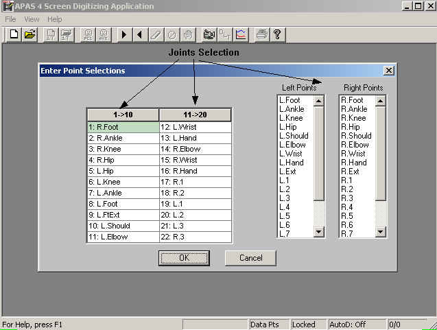
3.  Specify the Point Identifications

4.  Specify Control Point Coordinate Locations.

5.  Select Connect (Only If Point ID�s Have Been Changed)

The connect option should be used to re-connect the points anytime that the point information is changed.  When the Point ID�s are first entered, the APAS will automatically connect the points to form the body segments.  For example, the software knows that the Left Foot connects to the Left Ankle and the Left Ankle connects to the Left Knee etc.  This information is saved in the Sequence file.  If these points or connections are changed at anytime, the saved information is updated by selecting the Connect option.

6.  Select OK.  You are now ready to Open a New View within the Sequence.  Up to nine views can be used to analyze a single sequence, however, only four views can be opened simultaneously.

   Figure 4a. shows some of the available "models" that come standard with the APASlite:

Figure 4a.  Models for templates input

   After input the proper information, Figure 5 shows the results:

Figure 5. Sequence Parameters selected

   Looking at the #Points, Figure 6 shows the selected points to digitize:

Figure 6. Points ID selections.

7.  Specify Control Point Coordinate Locations.

Type the X, Y, Z coordinate values for each control point, pressing ENTER after each value.  Values must be entered in the units of measure selected for this sequence or incorrect results will be computed.  To display additional points that could not be displayed on the current page, select the MORE button.  The READ button allows the ability to read the control point locations from a previously digitized sequence.  When all values have been entered, check them a second time for accuracy.  Corrections may be made by pressing the ENTER key until the cursor is positioned over the desired value.  When all values have been entered correctly, select OK to accept the values and return to the Sequence Parameter menu.

8.  Select Connect (Only If Point ID�s Have Been Changed)

The connect option should be used to re-connect the points anytime that the point information is changed.  When the Point ID�s are first entered, the APAS will automatically connect the points to form the body segments.  For example, the software knows that the Left Foot connects to the Left Ankle and the Left Ankle connects to the Left Knee etc.  This information is saved in the Sequence file.  If these points or connections are changed at anytime, the saved information is updated by selecting the Connect option.

9.  Select OK.  You are now ready to Open a New View within the Sequence.  Up to nine views can be used to analyze a single sequence, however, only four views can be opened simultaneously.

   After inputting the Control Points, the data looks as in Figure 7.

Figure 7.  Control Points

   One must be very accurate in measuring the Calibration Frame in the view of the cameras. Any small error here will results in measurement error and erroneous results. 

   Every view, or camera needs to have a video image of the calibration frame in order to calibrate the view for the transformation process which create the 3D or 2D files.

   The next two figures show the Calibration Frame video frame and the associated measurement associates with each point which was digitized for the present demonstration.

Figure 8. Typical Calibration Frame.

Figure 9.  Measurements of the coordinates associated with the the Calibration Frame

   You can use any shape of calibration frame and choose any number of points. The minimum number points for 2D analysis are 4 planar points.  The minimum for 3D analysis you require to have at least 6 none co-planar points. Ideally, the calibration frame cover most the field of view. However, this is not a requirement. Some companies will try to sell you elaborate Calibration Frame configuration just to be able to charge you more money. Don't fall into this trap. Just make your own calibration frame exactly square and with standard measurement. Peak will sell you calibration frame for over $1000 and it cost them to make $25. What a steal and un-necessary.

   The next video will show step by step the material covered to this point:

All videos are highly compressed and do not represent the true video quality. When one use video cameras the digitizing files are presented in much better resolution.

Click here for Video View

  You may stop the video with the Media Player and advance it frame by frame to see all the steps up to this point.

Next Video as presented here

  shows all the steps to be able to load two simultaneously videos to the APASlite video screen to be ready for digitizing.

Next Video present all the steps to the digitizing process

OPENING A PREVIOUSLY CREATED PROJECT

1. Choose the SEQUENCE, OLD command from the FILE menu.  This can also be performed in a single step by selecting the OPEN EXISTING SEQUENCE icon from the Tool Bar.  The Open Existing Sequence menu box will appear.

2.  Select the desired sequence.

To Summarize this lesson

1.  You select the APASlite Icon as shown in the next Figure:

2. You Open the File Menu and select a new project as shown in the next Figure:

3. You define the new file. This is the .cf extension file as shown in the next Figure:

4.  Then, you input the Sequence Information such as the joints you are going to digitize, and the Calibration Frame Coordinates as shown in the next Figure:

5. Next Figure show the Point ID's for this particular project:

6.  The next Figure illustrates the Coordinates of the particular calibration frame:

7.  In the next Figure you shown the menu for selecting the view. Each camera is associated with a new view. You must input the Frame Rate for this camera. The Camera ID and the Camera location on the x,y,and z coordinates are not required.

8. After selecting the View and its associated video file you see the next Figure:

9. You may select another view to be able to digitize two views simultaneously. (With the regular APAS you may digitize up to 4 view simultaneously). 

   In the next lesson we will cover the actual digitizing process.

A very comprehensive descriptions of all the steps described so far available from the Digitizing Module at the regular APAS here.

Frame Rate - The Frame Rate is the number of images per second that are captured in the image file.  This item is always required and should be as accurate as possible in order to yield accurate velocity and acceleration computations.  For most APAS applications, the Frame Rate can be calculated by dividing the video speed by the sum of the skip factor plus one.  For example, if 300 images were captured from a 60 Hz video system with a skip factor of 1, the Frame Rate will equal 30  since ((60 / (1 + 1)) = 30 Hz.  Refer to the chart below for additional examples.

# Images       #Skip           #Images                         Frame Rate

300            0                300 / (0+1) = 300         60 / (0+1) = 60 Hz

300            1                300 / (1+1) = 150         60 / (1+1) = 30 Hz

300            2                300 / (2+1) = 100         60 / (2+1) = 20 Hz

300            3                300 / (3+1) = 75          60 / (3+1) = 15 Hz

Camera ID - Camera ID is an optional field provided to identify the type of camera used to record this view. 

Camera X, Y, Z - Camera X, Y, and Z defines the coordinate values for the location of the camera in the frame of reference of your control points.  The camera location is not required information to perform an analysis, however, if the location is known you may request a validity check of the transformation from digitizing space to image space.  This may be of value when publishing studies and demonstrating the validity of the method used.

View Type - View Type is used to specify each individual camera view as either STATIONARY or PANNING.  Stationary views are cameras that record the activity of interest from a �fixed� camera.  Fixed cameras can not be altered in any manner (zoomed, focused, moved etc) when recording the calibration points and activity data.  Panning views are cameras that record the calibration points and activity by Panning the camera from left-to-right or vice-versa.  As with the Stationary views, the zoom and focus should remain constant while recording the calibration points and activity.  Please refer to the PANNING CAMERAS section for additional information on digitizing panning views.

3.  Open the Image File

Select the Open PCX/AVI Images command from the File menu.  When this option is selected the Open file menu box will be presented.  Select the desired image file by entering the file name and pressing the ENTER key.  The Video File Information menu will be displayed. 

Select OK to proceed and display the first image in the AVI/PCX file in the active window.

4.  You are now ready to begin the Digitizing Process.  Please refer to the DIGITIZING PROCESS section for additional assistance.

JVC HIGH_SPEED CAMCORDER

When digitizing AVI files captured from the JVC 120 Hz Camcorders, there are a few extra points that must be emphasized.  The exact same steps are followed as described in the section �Creating A New Digitizing View File� with the following exceptions.

1.    The Frame Rate must be set to 120 or 240 (depending on the high-speed mode used for recording) in the View Information menu.

2.    Make certain that the SPEED field is labeled as 120 or 240.  If not, the file should be opened in TRIM module and specified as either 120 Hz or 240 Hz.  Then select the Save Trimming option without actually trimming the file.

3.  Select the CALIBRATE command from the IMAGES menu to display the Calibrate JVC 120Hz Offset menu.  It is recommended to select the AUTO button to automatically determine the image offset.  Select the OK button to return to the digitizing screen.

The JVC high-speed camcorder is capable of recording at a rate of either 120 or 240 images per second by splitting the image to approximately one-half or one-quarter normal screen size.  When the recording is played back on any standard video player, 2 images will be simultaneously displayed in the 120 Hz mode (2X High Density Mode) while 4 images will be simultaneously displayed in the 240 Hz mode (4X High Density Mode).  These images are 1/120^th second apart and 1/240^th second apart respectively.

In theory, the expected split would occur at the horizontal and vertical middle of the screen.  This equates to horizontal line 360 and vertical line 240 since there are 720 lines of horizontal resolution and 480 lines of vertical resolution.  However, reality has indicated that this is not always the situation.  For this reason, the Calibrate function is used to determine the image offsets for the high-speed video.

The steps for calibration are almost identical for both the 120 and 240 Hz modes.  Any of three options can be used to perform the calibration process, however, the �Automatic� method is recommended.  These options are selected using the buttons in the lower portion of the Calibrate menu.

Manual Calibration Option

In the �Calibrate� menu, the user specifies the row or column number (or both in the case of 240 Hz) where the last high speed image appears in the normal speed video.  In the case of 120 Hz, the normal video consists of 2 high speed images either horizontal scenes or vertical scenes.  In the case of 240 Hz, there are 2 rows and 2 columns of high-speed images per normal image. The dialog displays 2 images, the 1st and last high-speed images for the current normal image. Edit boxes display the current values for the row/column offsets for the "Last" image. The idea is to have the top or the left or both edges of the two displayed images appear identically. One can enter a value for the offset[s] and click on the �Apply� button to re-display the images with this new value.

Digitize Calibration Option

The �Digitize� option is another method for calibration.  When this option is selected, the user will be prompted to digitize the same image feature in the two images.  From this information the program calculates the row and/or column offsets.

Automatic Calibration Option

Or one can select "Auto" and the program will automatically compare the two images pixel by pixel and determine the row and/or column offsets.  The calculated offset is then entered in the Line Offset field. This last option is the most reliable and is the recommended method.  Typically the calibration needs to be performed only once on a system. The indicator that the 120/240 Hz is NOT calibrated is the presence of jitter when advancing images.

Save Calibration Settings

This information can only be saved to a file once. This usually happens in TRIM when the trimmed file is saved. Therefore this information should be setup properly before the trimmed file is saved. It can be changed temporarily but will revert to the original values the next time the AVI is opened. To save permanently, open the video file in the TRIMMER module, specify new values, and then save the trimmed file without actually trimming any images.

   [Go to lesson 2]  [Go to Index]