Kinematics

	Kinematics	[FrontPage Include Component]	Previous Home Up Next

NAVIGATOR: Back - Home > Adi > Services > Support > Tutorials > Gait > Chapter2 :

Kinematics

2.2 Principles of Gait Kinematics

	What is kinematics
	Degree of freedom
	Coordinate Systems: GCS and LCS
	Marker sets
	Anthropometry for marker sets
	Marker tracking to get 2D or 3D position
	Marker based LCS
	Joint center and segment axis estimation to get position and orientation of bones
	Joint angle calculation
	Principles of cardanic angle calculation, meaning, limitation, standardization
	Joint angle display and meaning of displayed joint angle
	Potential error from each step – can be included in each section
	Segment / joint angles, vel, acc (deg and rad) (2D and 3D)
	Force curves / parameters from the plates (This is normally not counted as kinematics, but for practical reasons it should be)

What is kinematics

Kinematics is the subdivision of mechanics that deals with the geometry of motion without regard to the forces causing the motion. Kinematics (and also Kinetics) considers each body segment as a rigid body and kinematics describes motion of each body segment in terms of displacement, velocity, and acceleration in space.

The kernel of kinematic analysis is to know the position and orientation of each body segment (rigid body) in space with respect to time. All of the kinematic variables can be derived from this information.

Linear displacement, velocity, and acceleration can be calculated from the position in space with respect to time.

Angular (rotational) displacement, velocity, and acceleration can be from the orientation in space with respect to time.

A geometry of motion can be described relative to the fixed, global (or laboratory) space or relative to another body segment (usually just proximal to the specific body segment). For convenience, we can call the former absolute kinematic data and the latter relative.

Twelve kinds of kinematic variables are generated from position and orientation data. (See table 3.1.1) Among these, the most widely used variable is relative, angular displacement, which is called joint angle. In clinical and most of research situation, relative linear displacement is ignored. Absolute angular and linear acceleration are the basic sources of kinetic (dynamic) calculation. Absolute angular displacement is used to describe the orientation of pelvis and feet. The pathway of center of gravity (CoG) is a kind of absolute linear displacement.

Table 3.1.1 Usage of kinematic variables.

	Linear (from position)			Angular (Rotational) (from orientation)
	displacement	Velocity	acceleration	displacement	Velocity	acceleration
Absolute	cog pathway		used for inverse dynamics	pelvis, foot orientation		used for inverse dynamics
Relative	usu. ignored			most of joint angles

Degree of freedom

Degrees of freedom (DOF) is the number of independent parameters required to completely characterize some system. We need 6 DOF - 3 translation (position) and 3 rotation (orientation) - to completely describe the motion of a rigid body in 3D space.

Coordinate system: GCS, LCS

Global coordinate system (GCS) is the frame with respect to which positional data of markers are provided by the stereophotogrammetric system. It is arbitrary chosen and usually coincides with the photogrammetric calibration object system.

The axes of GCS are usually defined as X, Y and Z according to right hand rule (hyperlink to show right hand rule with fig). International Society of Biomechanics recommended to define the X, Y and Z axes as below:

   X   coincides with the walking direction assigned to the subject and points anteriorly.
   Y   is orthogonal to the floor and points upwards.
   Z   goes from the left to the right-hand side of the subject.
   O   the origin must lie on the floor and on the midsagittal plane assigned to the subject.

Local coordinate system (LCS) is a Cartesian coordinate system fixed on a moving rigid body. To define the LCS of a rigid body, we should know the 3D positions (with respect to GCS) of at least three non-collinear points (markers). (hyperlink to show generation of LCS from 3 markers with animated figure) Without defining the LCS, we can not describe 3D movement of a rigid body in 6 DOF.

Marker sets

For gait kinematic and kinetic analysis, a number of markers are attached on specific locations of various body parts. Markers are tracked automatically by optoelectronic system to be represented as points in 3D space. After automatic tracking and 3D conversion, each marker has its own positional information/data in GCS. The configuration of specific locations of markers is called marker set. There are several conditions to be a good marker set.

Easy to track automatically

Should minimize the chance of hiding or merging of the markers

At least three noncolinear markers on a body segment

At least three markers are attached on a body segment

Can be reduced to 2 markers if we use virtual markers, such as joint center

For example, Helen Hayes marker set uses 13 or 15 markers for 7 body segments.

Able to define anatomically relevant LCS

To estimate joint centers accurately and to define anatomical planes (sagittal or coronal) of body segments should be warranted.

APAS/Gait can use 5 marker sets. Four marker sets among the 5 are the most widely used. And one is newly developed specifically for APAS/Gait.

Here are a brief description and a comparison table of the five marker sets:

1. Original Helen Hayes(HHo) marker set that used by Davis and Kadaba.
2. Modified Helen Hayes(HHm) marker set
3. Original Kit Vaughan's marker set(KVo) - published on his 1st edition of "Dynamic of human gait"
4. Modified Kit Vaughan's set (KVm) - published on his 2nd edition (CD ROM version)
5. Sun's marker set

* Comparison Table

* Marker sharing

** Marker Name and Position

Anthropometry for marker sets (Anthro for kinetics is not included)

** Body Segment Parameters to measure

Abbre	Full Name	Measurement	Used by
R,L LL	leg length	From ASIS to med malleolus	HHm, HHo
R,L Wkne	Knee width	From center of lat epicondyle to med. epicondyle	HHm, HHo
R,L Wank	Ankle width	From center of lat. Malleolus to med. Malleolus	HHm, HHo
R,L Vdis	Vertical distance	Vertical distance from GTRO to ASIS	HHm, HHo
m_offset1	Offset 1	Offset from bony landmark to center of larger marker* = radius of larger marker + thickness of plate + thickness of skin and subcut tissue	HHm, HHo, Sun
m_offset2	Offset 2	Offset from bony landmark to center of smaller marker = radius of smaller marker + hickness of plate + thickness of skin and subcut tissue	Sun
ASISW	ASIS width	Distance between bilateral ASISï¿½s	HHm, HHo, KVo, KVm
R,L malH	Malleolar height	Sole of foot to center of lat. malleolus	Kvo, KVm
R,L footL	Foot length	End of toe to heel	Kvo, KVm
R,L footW	Foot width	Width of metatarsal head area	Kvo, KVm
R,L MTHth	MT head thickness	Thickness of 2^nd metatarsal head	Sun, Kvo, KVm, HHm, HHo,
R,L H2GCMi	Heel to GCMi	Heel(bone) to GCM insertion (i direction)	Sun, Kvo, KVm, HHm, HHo,
R,L H2GCMj	Heel to GCMj	Heel(bone) to GCM insertion (j direction)	Sun, Kvo, KVm, HHm, HHo,
Beta	Beta angle	Angle from pelvis x ray analysis	HHm, HHo
theta	Theta angle	Angle from pelvis x ray analysis	HHm, HHo

* Normally use larger markers. Smaller markers are for medial epicondyle, medial malleolus and heel.

Joint center and segment axis estimation

*** Joint Center and bony landmarks Estimation

	Hip	Knee	Ankle
HHo	Davis	Direction: perpendicular line from thigh wand marker(R,LTHI_W) to the line between great. Trochanter marker (R,LGTRO) and Lat. Epicondyle marker (R,LLCON) Starting point: Lat. Epicondyle marker (R,LLCON) Amount: half of knee width(R,LWkne) + radius of marker	Direction: perpendicular line from tibia wand marker(R,LTIB_W) to the line between Lat. Epicondyle marker (R,LLCON) and Lat. Malleolus marker (R,LLMAL) Starting point: Lat. Malleolus marker (R,LLMAL) Amount: half of knee width(R,Lwank) + radius of marker
HHm	Davis	Direction: perpendicular line from thigh wand marker(R,LTHI_W) to the line between hip joint center and Lat. Epicondyle marker (R,LLCON) Starting point: Lat. Epicondyle marker (R,LLCON) Amount: half of knee width(R,LWkne) + radius of marker	Same as the above (HHo)
KVo	K.Vaughn	Specific point described by tibia marker based LCS (LCS from R,LCON, R,LTTUB and R,LLMAL)	Specific point described by foot marker based LCS (LCS from R,LMT, R,LHEEL and R,LLMAL) for KVo, they use 5^th MT head instead of 2^nd one.. But we used 2^nd one.
KVm	K.Vaughn	Direction: perpendicular line from tibia wand marker(R,LTIB_W) to the line between Lat. Epicondyle marker (R,LLCON) and Lat. Malleolus marker (R,LLMAL) Starting point: Lat. Epicondyle marker (R,LLCON) Amount: half of knee width(R,LWkne) + radius of marker	Same as the above(KVo) for KVm, they use 2^nd MT head instead of 5^th one.
Sun	Bell	mid point between Lat. Epicondyle marker (R,LLCON) and Med. Epicondyle marker(R,LMCON) – virtual marker	mid point between Lat. Malleolus marker (R,LLMAL) and Med. Malleolus marker(R,LMMAL) – virtual marker

Definition of Anatomical plane of each body segments (Anatomy based LCS)

	Pelvis	Thigh	Lower Leg	Foot
HHo	k: LASIS to RASIS i: perpendicular from SACR to k j = k ï¿½ i	j: from knee jc to hip jc k: perpendicular from j to RTHI_W or LTHI_W to j i = j ï¿½ k	j: from ankle jc to knee jc k: perpendicular from j to RTIB_W or LTIB_W to j i = j ï¿½ k	i: from R,LHEEL to R,LMT j: perpendicular from i to ankle jc k = i ï¿½ j
HHm	Same	Same as HHo	Same as HHo	same as HHo
KVo	Same	j: from knee jc to hip jc i = j ï¿½ (RGTRO- hip jc) or (LGTRO-hip jc) ï¿½ j k = i ï¿½ j	j: from ankle jc to knee jc i = j ï¿½ (RLCON- knee jc) or (LLCON-knee jc) ï¿½ j k = i ï¿½ j	basically same as HHo
KVm	Same	j: from knee jc to hip jc i = j ï¿½ (RTHI_W- hip jc) or (LTHI_W-hip jc) ï¿½ j k = i ï¿½ j	j: from ankle jc to knee jc i = j ï¿½ (RLCON- knee jc) or (LLCON-knee jc) ï¿½ j k = i ï¿½ j	basically Same as HHo
Sun	Same	j: from knee jc to hip jc k: perpendicular from j to RLCON or LLCON to j i = j ï¿½ k	j: from ankle jc to knee jc k: perpendicular from j to RLMAL or LLMAL to j i = j ï¿½ k	Same
New Sun	Same	j: from knee jc to hip jc i = j ï¿½ (RLCON-RMCON) or j ï¿½ (LMCON - LLCON) i = j ï¿½ k	j: from ankle jc to knee jc i = j ï¿½ (RLMAL-RMMAL) or j ï¿½ (LMMAL - LLMAL) i = j ï¿½ k	Same

* Normally use larger markers. Smaller markers are for medial epicondyle, medial malleolus and heel.

Joint center and segment axis estimation

Definition of Anatomical plane of each body segments (Anatomy based LCS)

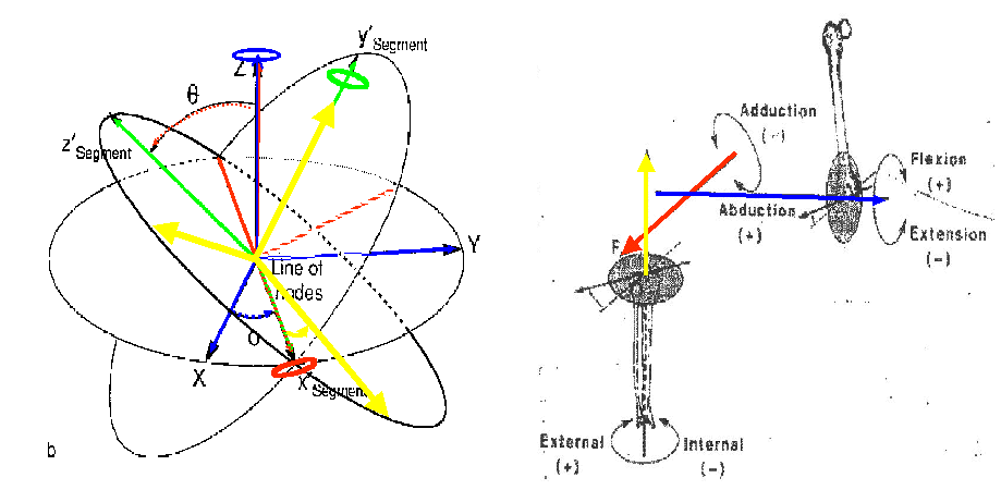
Joint Angle Calculation (NJCS)

- Nonorthogonal Joint coordination system based on Euler/Cardanic convention

Flexion/Extension angle : 1^st rotation about k of proximal segment

Adduction/Abduction angle : 2^nd rotation about coperpendicular vector between proximal k and distal j.

Int/Ext rotation angle: 3^rd rotation about j vector of distal segment

This page was last modified on 12/07/2008 at 22:47 PST. Copyright ï¿½ 1994 - 2002, all rights reserved, Ariel Dynamics Inc. Please send your comments or feedback to webmaster@arielnet.com or proceed to our feedback form. This page has been accessed many times since Dec 12, 2002. Our privacy policy is here.