|
|
Analog |
[FrontPage Include Component] |
|
|
|
|
|
|||||
|
NAVIGATOR: Back - Home > Adi > Services > Support > Manuals > Apas > Dos : |
|||||
|
|
|||||
| |||||||||||||||||||
|
Analog
Categories
|
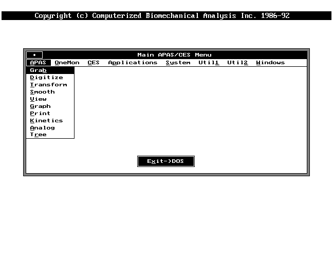
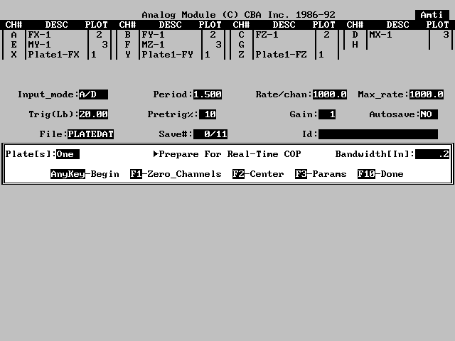
ANALOG MODULE14.1 ANALOG PROCESS The Analog Module is used as a general purpose laboratory data measurement and analysis subsystem. The module is designed to sample, save and present analog signals from up to thirty two independent channels. An aggregate measurement rate of up to 20,000 samples/second is possible, with input voltage ranges of -5 to + 5 volts (or -10 to +10 volts). Data signals are measured to an accuracy of 0.025% of the full scale voltage range. A number of triggering options are provided to assist in the capture of transient data and to allow the synchronization of the analog module with external events. The analog module also includes a set of specialized electromyogram (EMG) signal processing options. EMG data samples can be analyzed using a number of sophisticated techniques including spike analysis, signal rectification and integration, envelope processing and spectral analysis. The Analog Module is selected from the Main Analysis Menu. The first screen shows system resource information. This menu is for informational purposes only. "Board Type" specifies the type of analog board currently installed in the computer. "Max Rate" specifies the maximum rate the analog board can handle. This number should be divided by the number of channels for the maximum Rate/Channel value. "Buffer Size (MB)" specifies the size, in Megabytes, of the memory buffer. "Free Disk (MB)" specifies the available memory, in Megabytes, on the current hard disk drive. This number should be checked prior to data acquisition to ensure there is enough room for the data being taken.Any Key may be pressed to proceed into the Analog Module. The Main Analog Menu has six various options for use in the analog process. At the top of the screen is the Analog Channel Table with the active analog channels. Channels are designated by letters, starting with A for the first channel, B for the second and so on. Each channel represents a separate input signal on the hardware analog interface. Up to thirty-two channels or signals may be processed by the Analog Module. The number of channels and the individual channel descriptions may be selected through Options selection. Analog input is controlled by the analog sampling parameters that are displayed above the menu box. These parameters must be set before the Analog Module may process the analog measurements. Thus, these options will be discussed before the analog measurement process which is discussed in Subchapter 14.6, Analog Measurement Process. Analog input signals and channel definition will be discussed in Subchapter 14.10, at the end of this chapter. 14.1.1 F1_COP The F1 key selects the Real Time Center-Of-Pressure (COP) option . This option requires at least one force plate.
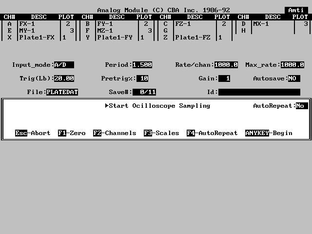
14.1.2 F2_Scope The F2 key selects the Real Time Oscilloscope option. This option is useful for examining data as it is being sampled.
When scope sampling is completed, pressing any key on the keyboard will return to the Start Oscilloscope Sampling Menu and ready the system for another sample to be taken. F1-Data Analysis will return to the Analog Data Processing Menu. F10-Done will return to the Main Analog Menu. 14.1.3 F3_Vectors The F3 key selects the Real Time Force Vectors. This option requires at least one force plate and a video input source and allows vertical force plate vectors to be superimposed on a live video image.
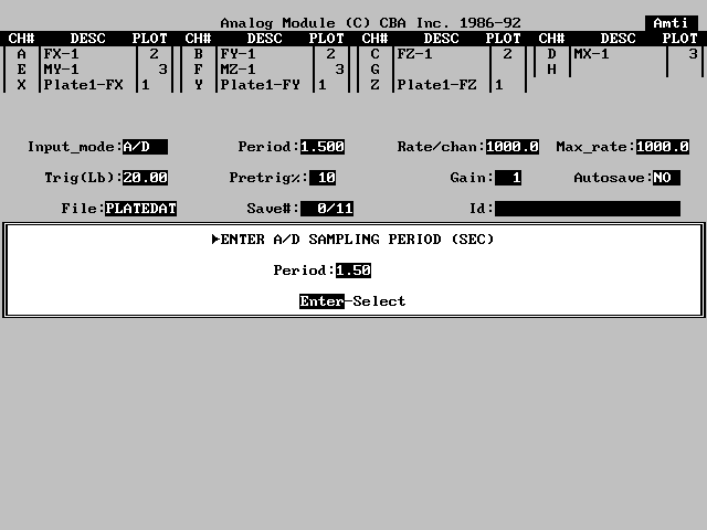
14.2 SAMPLE The Sample option is selected to initiate sampling of the analog data channels. The analog input is controlled by the analog sampling parameters that are displayed above the menu box on the monochrome screen. These parameters must be set before the Analog Module may process the analog measurements. Thus, because the Sample option is used to initiate the analog measurements and all other options of the Main Analysis Menu are used to set these sampling parameters and prepare the module for sampling, the Sampling option will be discussed later in Subchapter 14.8, Analog Measurement Process and the other options will be discussed first in the next subchapters. 14.3 PERIOD Period is selected to set the duration of analog measurement. The sampling period is the length of an analog sample in seconds. All the active analog channels are measured continuously over the sampling period. The number of analog measurements that are performed for each channel during the sampling period is determined by the sampling rate or Rate/Chan. The sampling rate is the number of data measurements per second for each analog channel. The total number of data values sampled and saved is the sampling period times the rate/channel times the number of channels. Thus, if 1000 is entered in Rate/Chan and 2 is entered in Period then 2000 data values are collected for each channel during the sampling period. If there are eight active channels, then a total of 16,000 data values would be collected each time analog sampling is performed. The Analog module can collect a maximum of 32,000 data values at one time. If the sampling period times the sampling rate times the number of channels exceeds 32,000 then the sampling rate (Rate/Chan) will be automatically reduced to stay within the maximum number of data measurements. When specifying a sampling period, it is best to select a period that is long enough to encompass the entire activity, but not so long as to collect a large number of unnecessary data measurements. Some experimentation may be necessary when setting up for analog data collection to determine the optimum sampling period. In a similar manner, the sampling rate should not be set to a higher value than necessary for the type of signal being measured. The Rate/Chan is set through the Options selection on the Main Menu. 14.4 TRIGGER The Trigger option is used to set the parameters relating to the triggering event. Triggering is a technique whereby the level of the analog signal being measured is used to determine the start of the sampling period. These include the trigger channel, the trigger level, and the pretrigger percent. For example, if the measurements of a running stride are being made using a force platform, one could observe the subject approaching the platform, and then manually initiate sampling just before foot contact occurs. Unfortunately, experience has shown this to be an unreliable method of data collection as there is too much chance of starting the measurement too early or too late and thus missing some of the activity being studied. A more reliable method is to use the analog signal from the force platform resulting from the initial foot contact to mark the beginning of the sampling period. This illustrates the concept of a triggering event. Frequently, one wishes to start analog measurement before the actual triggering event occurs. In the example above, by the time the foot contact signal reaches a level sufficient to trigger analog sampling some of the low level initial contact forces have been missed. A pretrigger analog sampling some of the low level initial contact forces have been missed. A pretrigger is a technique whereby a number of the most recent analog measurements are saved while awaiting the triggering event. This is accomplished using a circular buffer in which the most recent samples replace the oldest ones. When the trigger occurs, measurement continues to the end of the sampling period. then the desired number of pre-trigger measurements are copied from the pretrigger buffer yielding a continuous analog sample starting at some time before and ending at sometime after the triggering event. The trigger parameters on the Trigger Parameter Screen are:
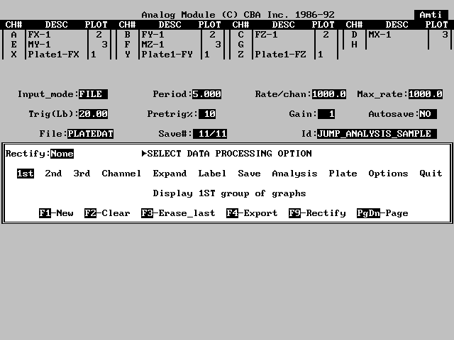
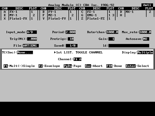
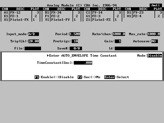
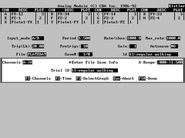
In addition, the current data file may be converted to "DIF", "WKS" or "ASCII" format for interchange with other software programs. Each analog sample, the measurements for one sampling period, is saved in a separate record in the file. As additional samples are saved they are added to the end of the current file. Up to 100 individual samples may be saved in a single analog data file. The number of the current analog file record is shown in the Save# item in the parameter area. Individual data records cannot be deleted without deleting the entire file. 14.5 MODE Up to this point, the measuring and saving of analog data values have been discussed. This is the initial or default mode of the analog module and is called A/D mode because actual analog to digital conversion is performed. This mode indicator appears in the Input_mode field in the parameter area. To access previously saved analog samples, the input mode must be changed to the File Mode so the analog values will then be read from the desired file. This is done using the Mode option on the Main Analog Menu. In the File mode, analog sampling cannot be performed using the analog to digital interface. The Sample option on the Main Analog Menu is replaced by the Retrieve option. This option allows previously sampled and saved data to be read or retrieved from a data file. When Retrieve is selected, one may Advance to the next saved sample in the file or Backup to the previous saved sample or Select any particular saved sample. The Select option will display a list of all sample ID's in the file to facilitate sample selection. When a saved sample is read, the information is displayed in the same manner as when analog sampling has been performed. The analog processing menu appears on the monochrome monitor, and analysis of this sample may then take place. It is possible to change between A/D mode and File mode at any time. For example, if data is being sampled and saved in a file, in the A/D mode, it is possible to review previous samples by selecting File mode and reading the desired sample. Similarly, if previously sampled data is being examined, in the File mode, it is possible to add new data to this file by selecting A/D mode and performing additional sampling of analog signals. New data is always saved at the end of a file so that previously saved data is retained. 14.6 DISPLAY Display is selected from the Main Analog Menu to either add or remove one of the three plot_lists of the analog channels or change the colors of various items on the color monitor such as curves, axis, logo or background. 14.6.1 Plot_Lists Plot_lists are merely lists of analog channels that are plotted or graphed together. By grouping channels in this manner, time is saved in the display and analysis of analog input. The first plot_list is automatically graphed after each analog sample is collected or read from a file. The other plot_lists may be graphed by selecting the "2nd" and/or "3rd" options on the analog processing menu. The "Plot" column in the channel table shows which plot list(s) each analog channel is associated with. The three lists are designated by the number 1,2 and 3. A channel may be on more than one plot_list, if desired. since the first plot_list is automatically graphed when analog input is performed, it is recommended that as many of the input channels be assigned to this list as is practical. Channels with different units should be assigned to separate plot_lists, as graphs are labeled with the units of the first channel plotted. The menu box lists all the analog channels. A channel is selected by simply pressing the letter key for that channel or highlighting the channel letter and pressing ENTER. A channel that is currently selected may be removed from this plot_list by selecting that channel letter again. The plot_list assignments are shown in the channel table at the top of the monochrome screen under the "PLOT" heading. A 1 indicator is used for the first plot_list, and 2 for the second, and a 3 for the third. A channel may be on more than one list at the same time. 14.6.1.1 F1-Multiple Single A plot_list is normally displayed in "Multiple" mode. In this mode all channels on the list are drawn on a single graph. Alternately, a plot_list may be displayed in "Single" mode. In this mode each channel on the list is displayed on a separate graph. This option is often used for rapidly fluctuating data such as EMG signals. The mode of the current plot_list is shown in the upper right corner of the menu box and may be changed by pressing the F1_Multiple/Single key. Each time F1 is pressed the mode is toggled to the other display mode. 14.6.1.2 F2-Envelope As an additional option, Automatic Envelope Processing may be selected for a plot_list. When this option is selected (usually when EMG signals are being processed), and envelope curve will be graphed for each data curve on this plot_list. To select this option, press the F2-Envelope key and enter a time constant for the envelope curve. The time constant is shown in the upper left corner of the menu box. A value of "None" indicates that the automatic envelope option is not selected. 14.6.2 Colors Colors is selected when the color assignment for one or more of the display items is to be changed. Color selection may be performed for each of the data curves (up to nine on a single graph), the graph axes, the logo (text at the top of the display), and the display background. Each item may be set to any of the sixteen available colors. Be aware that items set to the background color will disappear. they may be seen again by setting the color to another value.
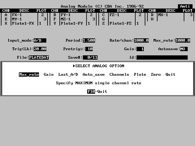
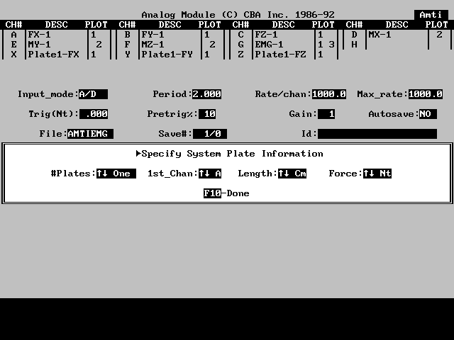
14.7.1 Max_Rate The Max Rate is used to set the maximum sampling rate for a single analog channel. The maximum rate is used to calculate the actual sampling rate, Rate/Chan that appears in the analog sampling parameters. In most cases, the actual sampling rate will be the Max_Rate value. However, certain conditions will result in a smaller Rate/Chan value being used. The first condition is when the aggregate sampling rate (number of channels times Max_Rate) exceeds the maximum hardware sampling rate (20,000 samples/second with a single channel maximum of 5,000 samples/second) the "Rate/Chan" will be reduced automatically to adjust to the maximum hardware limit. If this latter condition occurs, the Rate/Chan value may be increased by decreasing the sampling period. 14.7.2 Gain Gain is used to set the programmable gain on the analog input module. The current gain is shown in the Gain field in the analog sampling parameters. The initial or default gain is 1 (no signal amplification), which results in an analog input range of + 10 volts and a resolution of approximately 5 millivolts. for low level input signals, the gain may alternately be set to either 10 or 100. A gain of 10 gives an analog input range of + 1 volt, and a resolution of approximately 0.5 millivolts. A gain of 100 gives an analog input range of +100 millivolts and a resolution of approximately 50 microvolts. when a gain of 100 is used, an optional capacitor must be connected to the analog converter to increase settling time. This, in turn, decreases the maximum aggregate sampling rate to 20,000 samples/second. If only higher level analog signals will be processed, the analog module may optionally be equipped with a programmable amplifier having gains of 1, 2, 4 and 8 rather than the above mentioned 1, 10 and 100. 14.7.3 Last_A/D The Last_A/D field is used to select the number of active analog channels. Since the active channels always begin with channel A, the number of channels are set by specifying the last active channel. The active analog channels appear in the channel table at the top of the screen. The number of entries in this table are determined by the value of the Last_A/D channel. One should not specify more channels than the actual number of analog input signals, as any additional empty channels will waste input buffer space and possibly cause the sampling rate to be reduced. 14.7.4 Auto_Save Auto_Save is used to specify analog channels that are to be automatically saved to the current data file whenever a new sample is requested. Normally, a Save command must be issued to cause the analog values to be saved in order to prevent unwanted data from being written to the file. In some situations where a number of consecutive analog samples will be measured, automatic saving of data is selected to insure that samples are not inadvertently lost through human error. The current status of the Autosave feature is indicated in the analog sampling parameter area on the monochrome monitor. No indicates that this feature is not selected, while Yes indicates that autosave is selected. 14.7.5 Channels Channels is used to set or change the individual analog channel definitions in the analog channel table. When this option is selected, a table of the analog channels is displayed. Any channel description (name), units, conversion factor (units/volt of analog signal), and offset (signal level in volts corresponding to zero in the units of that channel) may be entered. The current channel settings are saved each time the analog module is exited so they do not have to be reset the next time the module is run. In addition, each time an existing analog data file is accessed, the channel definitions are copied from that file. In this manner, different sets of channel definitions corresponding to different types of input (force platforms, EMG equipment, etc.) can be quickly accessed from a predefined data set. The rest of this option discussion has been deferred to the end of this chapter, Sub-Chapter 14.9, Analog Signals and Analog Channel Definition section, to allow the specific features of the analog module to be resented without having to be concerned with the actual source of the analog signals. In practice, the first item to be considered in the data collection process is the source, type, and magnitude of the individual analog signals along with the corresponding definition of the analog channel table. 14.7.6 Plate Plate is used to define special force platform (force plate) processing by assigning a block of analog input channels to predefined force platform signals. Typical biomechanical force platforms have six to eight analog outputs representing forces and moments measured directly by the platform. These outputs are frequently combined or used to compute additional quantities such as composite forces, moments, and point of application of force. Rather than require a user to set up numerous input channels, the Plate option automatically defines a consecutive group of channels as standard force platform input for the type of platform configured with this system (various platform definitions supporting most commercially available force platforms can be configured when the system is ordered). In addition, since the channel definitions are predefined, the computed quantities are also automatically defined and displayed as additional analog channels. When Plate is selected the starting channel for the force plate signals must be indicated. The analog module will then show the expected force plate inputs and channel assignments for the type of plate configured to the system. Once configured, all measured and computer force plate quantities are available for graphing and analysis. 14.7.6.1 Info Info is selected to specify general force plate system information. the information asked for is dependent upon the type of force plate being used. 14.7.6.2 1 Plate 1_Plate is selected to enter parameters for each force plate. the information asked for is dependent upon the type of force plate being used. 14.7.6.3 2 Plate 2_Plate is selected to specify the relative positioning of multiple force plate systems. Additional help is provided at the subsequent data entry form. 14.7.6.4 Electronics Electronics is selected to enter the force plate amplifier information. the information asked for is dependent upon the type of force plate being used. 14.7.7 Zero Zero is selected to determine the zero levels for the input channels and the analog-to-digital converter. 14.7.7.1 Channel Range The Channel_Range is selected to determine zero levels for the analog input channels. the determined zero levels are used by the software to insure that the input analog values are properly zeroed. this option should be periodically executed to insure against zero drift. The analog systems should always be allowed time to warm up before using and zeroing. Enter the first and last channels for auto-zeroing. Acceptable values are scrolled through using the up and down arrow keys. Typically, all input analog channels are selected including force plate and EMG data. Press ENTER to proceed to the last channel choice. After selecting the last channel, press F10 to return to the previous menu. Make sure that the channels are at the zero level. For force plates, the zero level corresponds to an unloaded force plate. 14.7.7.2 A/D The A/D Converter is selected to calibrate the analog to digital converter. Short circuit the input to the specified channel then strike any key to calibrate the A/D converter. Short circuiting the channel is best accomplished with a BNC shorting plug available from any electronics supplier. A summary table of A/D values for specific gain settings is displayed for informational purposes. The "New" values have been computed and can be compared to the previous settings listed as "Old" values. A/D values listed as NA for a gain of 2 or greater indicates that the analog board does not have a programmable gain option. Pressing any key on the keyboard will return to the Zero Calibration Function menu. 14.8 ANALOG MEASUREMENT PROCESS (SAMPLE) Once the analog sampling parameters have been set to accommodate the signals being measured, actual analog sampling may begin. The most recent values of the sampling parameters are saved and are reset when the module is run again. Thus sampling parameters do not need to be set each time analog processing is begun unless sampling values must be changed. The Sample Option on the Main Analog Menu is used to initiate analog measurement. When Sample is selected, the analog module displays a reminder message to prepare for analog measurement. At this point actual sampling has not begun and two options are available. The first option is to begin analog sampling by pressing any key on the keyboard. The second option is to abort by pressing the F10 key to return to the Main Analog Menu. The purpose of this additional step is to allow a final check of the analog signal source, force platform. EMG equipment, etc., and make sure that the subject is prepared to perform the activity being measured. As soon as analog input is "armed", the analog module begins measuring each of the input signals and monitoring the trigger channel for the triggering event. A message will appear on the screen to indicate that analog sampling is taking place. Sampling may be aborted at this time by pressing any key on the keyboard. The abort option is provided in the event the subject is not able to perform the activity, equipment malfunction, or there is an interruption in the normal sampling process. Abort will return the screen to the Main Analog Menu. Assuming that sampling has occurred normally and that the triggering event has been detected, analog sampling will end when all of the post trigger measurements have been collected. The Analog Module will sound an audible "beep" to mark the end of data collection and the measured analog signals will appear on the color graphic display. The display is in graph format with the horizontal axis corresponding to the sampling period (time), and the vertical axis corresponding to the units of measurement of the analog signals. The signal from each channel is displayed as a curve with different colors being used to distinguish different channels. After sampling has been completed the Analog Data Processing Menu is displayed. This is the primary menu used for the display and analysis of data in the Analog Module. Some of the listed options are used to display analog data measurements in different ways, while other options provide various types of data analysis functions from simple measurement of values and intervals to sophisticated signal processing. Included in these analysis functions are a number of specialized EMG processing applications. A discussion of these display and analysis options will be the subject of the following sub-sections. 14.8.1 Function Keys The Function keys, whose definitions are shown at the bottom of the menu box of the Data Processing Option Menu, allow additional options that are used in the selection of the current graph. 14.8.1.1 F1 New Before plotting individual analog channels, one typically creates a new (empty) graph as the current graph. To start a new graph from the Analog Data Processing Menu, the F1-New key is pressed. The existing graph(s) are moved up on the display and space is created for a new graph at the bottom of the display. Any number of curves may now be drawn on this graph using the Channel option. 14.8.1.2 F2 Clear Alternately, one may wish to clear all the graphs on the display so that the new graph will be drawn using the full display screen. This is accomplished using the F2-Clear key. 14.8.1.3 F3 Erase Last A third option allows the current graph to be replaced with a new graph, while leaving the previous graphs on the display. This option is selected by pressing the F3-Erase_Last key. The last graph is cleared and the space it occupied may then be used for a new graph. If Erase_Last is selected more than once, the last or lowest previous graph will be erased and the display will be redrawn with all remaining graphs enlarged and one new empty graph area at the bottom of the display. 14.8.1.4 F4 -Export The F4_Export key selects one additional graph related option. This key is used to produce table prints of numerical curve values from the current graph. When this option is selected you will be asked to indicate a horizontal interval on the current graph. A table will then be printed on the printer with values from each of the data curves on the graph for that interval. Since typical analog sampling contains hundred and perhaps thousands of measurements for each channel, the table print will reduce the number of values printed by selecting data points at measured intervals along the curves. To complete the table print command a skip factor must be entered for use in printing the data values. Since the Analog Module may measure thousands of values for each channel it is normally not practical to print all values in a table. the skip factor is used to specify the frequency of values to be printed. A factor of 1 would cause every value to be printed. A factor of 2 would cause every other value to be printed. A factor of 10 would cause every tenth value to be printed, and so on. If in doubt, start with a factor of ten and adjust accordingly.
14.8.1.5 F9 Rectify The F9_Rectify is selected to set or change the rectification mode used on the raw data. The current rectification mode is shown in the upper right corner of the menu box. The choices for rectification are "None" (for no rectification) "Half_Wave" and "Full_Wave". EMG signals are usually integrated using "Full_Wave" rectification.
In order to simplify the process of determining which channels are to be drawn on which graph, the Analog Module contains a feature called the Plot List. This is simply a list of analog channels (from one to nine) that are to be drawn on a single graph. Three plot lists can be defined in the analog module and they are designated the 1st, 2nd and the 3rd. After each analog sample is collected, or when previously sampled analog data is read from a file, the first plot list is automatically graphed. This is the initial display that appears along with the analog processing menu. If only a few analog channels are being measured, a single plot list is probably sufficient to display all active channels. In this case, all channels are automatically displayed after each sample. For larger numbers of channels, or if values for different channels are expressed in different units of measurement (the units for each graph are those of the first channel plotted on that graph), two or three plot lists should be used. In this case, more than one graph will be required to display all the analog data. The Analog Data Processing Menu allows any of the plot lists to be added as an additional graph on the current display through the 1st, 2nd and 3rd options. Each time one of these options is selected a new graph is drawn to display the channels from that plot list. As mentioned, the first plot list is graphed automatically. The second plot list is graphed using the 2nd option, and the third plot list using the 3rd. In this manner, many analog channel curves can be quickly graphed for examination and analysis. 14.8.3 Channel Plot lists are used to graph groups of channels. In addition, the Analog module allows any single active analog channel to be graphed using the Channel option. When Channel is selected, a list of active channels is presented. Choosing a channel letter will cause the data curve for that channel to be added to the current graph. In this manner, graphs may be created with curves for one or more analog channels in different combinations than the ones defined for the three existing plot lists. The active analog channels are displayed in the menu box. To select the channel to be added as an additional curve on the current graph simply press the letter key corresponding to that channel. 14.8.4 Expand The Expand option is selected to expand the current graph so that a horizontal and/or vertical interval of the existing curves is expanded and plotted to the full scale of the graph. This is essentially a zoom function that allows any portion of the current graph to be examined in an enlarged format. When this option is selected the horizontal or vertical interval must be specified either by using the mouse or by typing the endpoint values of the interval. The graph may then be redrawn for this interval, thus performing an expansion of the original graph. Expand may be selected repeatedly, each time specifying an interval on the already expanded graph. In this manner even the smallest detail recorded may be zoomed in. The usefulness of the expand option becomes apparent when considering that the maximum resolution of the graphic display is 640 points horizontally and 400 points vertically. Analog signals, if recorded to the full input scale, have a resolution of about 4000 units vertically and several thousand units horizontally, depending on the sampling rate and period. To visually observe the smallest detail capable of being measured and recorded, data curves must be expanded. Analysis will not always require this level of detail, and frequently unexpanded curves are sufficient to provide the necessary data measurements.
In addition to providing standard text labels for annotation of analog displays, the labeling options perform various computations on the data values in individual curves and report the results of these computations in label format. In this manner basic analysis and labeling of data curves can occur simultaneously. 14.8.5.1 Normal Normal labels are text labels entered at the keyboard. Any character string can be added to the display in one of four text sizes and one of a number if colors. Labels may be positioned to any screen location using the mouse. this option is identical to the Label option in the Viewing and Graphing Modules. After Normal has been selected the screen will ask for the Text Label to be added to the display. The F1_Size key and F2_Color key are used to change the size and color of the labels, this must be done before the label is typed in. Any forty character label may be typed in and ENTER must then be pressed to accept the label. At this point the mouse is used to position the label to the desired location of the screen.
14.8.5.3 Range As with Value, the Range labels report horizontal or vertical graph intervals. Horizontal (X) intervals are measured in seconds, while vertical (Y) intervals are measured in the units of the graphed curves. the mouse is used to enter the endpoints of the interval to be reported by selecting the first point and pressing ENTER and then selecting the second point and pressing ENTER again. To select the entire data range press the F1_Whole_Range key. Alternately, the numeric range may be specified by pressing the F2-Numeric key and typing the starting and ending values for the range. The interval value then appears in the label text field. The F1_Size key and F2_Color key are used to change the size and color of the labels, this must be done before the label is accepted by pressing the ENTER key. At this point the mouse is used to position the label to the desired location on the screen. When this label is positioned on the display, a line will connect the beginning of the label to the indicated point. This option is typically used to measure the width (X interval) or height (Y interval) of individual features on the analog data curves. 14.8.5.4 Integral Integral labels report the area or integral under individual data curves. the units of measure are the product of the curve units and time. for example, if the data curve is measured in pounds (perhaps a force platform measurement), then the integral of this curve would be reported in pound-seconds which is a measure of impulse or the net change in momentum. The menu box contains a list of the active channels displayed on the current graph. To select the channel to be used simply highlight the channel name and press ENTER or press the letter key corresponding to that channel. channels are identified on the graph by channel letters displayed in the same color as the graphed curves. Only channels on the current graph may be selected for labeling. The mouse is used to enter the endpoints of the interval to be reported by selecting the first point and pressing ENTER and then selecting the second point and pressing ENTER again. To select the entire data range press the F1-Whole_Range key. Alternately, the numeric range may be specified by pressing the F2-Numeric key and typing the starting and ending values for the range. The interval value then appears in the label text field. the F1_Size key and F2_Color key are used to change the size and color of the labels, this must be done before the label is accepted by pressing the ENTER key. At this point the mouse is used to position the label to the desired location on the screen. When this label is positioned on the display, a line will connect the beginning of the label to the indicated point. 14.8.5.5 Average Average labels report the average value of individual data curves over a specified horizontal interval. the units of measure are the units defined for that analog channel. As with the Integral labeling option, the menu box for the Average option contains a list of the active channels displayed on the current graph. To select the channel to be used simply highlight the channel name and press ENTER or press the letter key corresponding to that channel. Channels are identified on the graph by channel letters displayed in the same color as the graphed curves. Only channels on the current graph may be selected for labeling. The mouse is used to enter the endpoints of the interval to be reported by selecting the first point and pressing ENTER and then selecting the second point and pressing ENTER again. To select the entire data range press the F1-Whole_Range key. Alternately, the numeric range may be specified by pressing the F2-Numeric key and typing the starting and ending values for the range. The interval value then appears in the label text field. The F1_Size key and F2_Color key are used to change the size and color of the labels, this must be done before the label is accepted by pressing the ENTER key. At this point the mouse is used to position the label to the desired location on the screen. When this label is positioned on the display, a line will connect the beginning of the label to the indicated point. 14.8.5.6 Slope Slope labels report the slope of individual data curves at a specified point. the units of measure for slope values are data curve units/second. The menu box contains a list of the active channels displayed on the current graph. to select the channel to be used simply highlight the channel name and press ENTER or press the letter key corresponding to that channel. Channels are identified on the graph by channel letters displayed in the same color as the graphed curves. Only channels on the current graph may be selected for labeling. The mouse is used to enter the endpoints of the interval to be reported by selecting the first point and pressing ENTER and then selecting the second point and pressing ENTER again. The interval value then appears in the label text field. The F1_Size key and F2_Color key are used to change the size and color of the labels, this must be done before the label is accepted by pressing the ENTER key. At this point the mouse is used to position the label to the desired location on the screen. When this label is positioned on the display, a line will connect the beginning of the label to the indicated point.
14.8.5.7 Min/Max
Min/Max is selected to label the Minimum and Maximum value for the data curve.
14.8.5.8 Onset
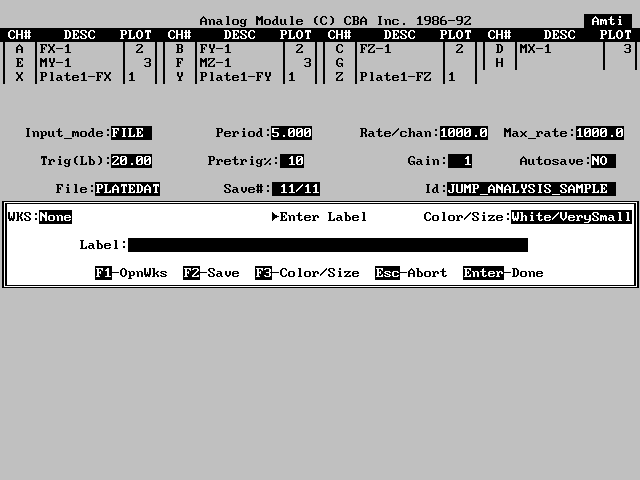
When Save is selected the Save Screen will appear asking for an ID for the file. Once an ID is typed in and F10-Save key pressed, the data will be written to the active data file. Alternately, the ESC key may be pressed to abort the save option. There are several options that may be performed when analog samples are saved to allow identification of the sample and to limit the amount of data that is actually saved.
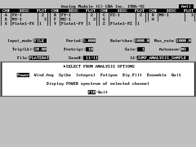
EMG signals are made up of numbers of individual pulses or spikes resulting from the firing of individual muscle motor units. Different motor units fire at different rates resulting in a composite EMG signal that is the sum of individual signals at varying frequencies. Classical numerical methods, such as Fourier analysis, can be applied to the composite signal to estimate the component frequencies. When either the Power, Envelope, Spike or Integral option is selected, a menu box containing a list of the active channels, displayed on the most recent graph of measured analog values may be selected for power spectrum analysis. Select the desired channel by highlighting the channel name and pressing ENTER or selecting corresponding channel letter.
For EMG signals, this is typically a pulse train or interval of significant motor unit activity. A new graph will be drawn with the power spectrum curve for this analog channel. If additional power spectra are computed, they will be drawn on this same graph and labeled with the analog channel name. Only the power of component frequencies below the cutoff will be reported. This allows the power spectrum to be scaled to the frequency of data measurement (Rate/Chan).
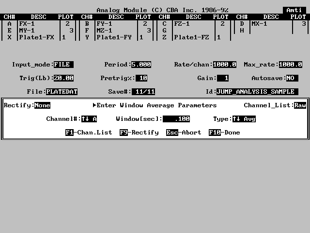
Lower frequency range may be selected if higher frequencies are not present in the data. This yields greater resolution on the power spectrum curve. For example, EMG data may be sampled at 1000 samples/second (Nyquist frequency of 500Hz), but component EMG signals are almost always below 200 Hz. By selecting a maximum frequency of 200 Hz, the power spectrum curve will show more than twice the resolution of a curve with a maximum frequency of 500 Hz. The mouse is used to enter the endpoints of the interval to be reported by selecting the first point and pressing ENTER and then selecting the second point and pressing ENTER again. To select the entire data range press the F1-Whole_range key. Alternately, the numeric range may be specified by pressing the F2-Numeric key and typing the starting and ending values for the range. 14.8.7.2 Wind.Avg. Because of the rapidly varying nature of EMG signals, averaging methods are frequently employed to simplify or smooth the curves for analysis. Window average (Wind.Avg.) analysis is selected to compute a linear envelope of an analog input signal using the moving window average method. This type of analysis produces a data curve value at time (t) with the average of the curve values over the interval or window form t-T/2 to t+T/2, where T is the interval time or "window width". the Envelope option allows the specification of T so that averaging may be tailored to differing individual applications. this type of analysis is often applied to EMG signals to remove the high frequency "spikes" while retaining the overall shape of the EMG curve. Window average processing may, however, be applied to any type of analog signal, not just to EMG signals. Typical values for standard EMG signals range from 10 ms to 30 ms. The moving window average method of computing envelopes is superior to analog low-pass filters often employed in EMG analysis, as analog filters introduce a phase lag in their output. When Wind is selected, the curve to be averaged must be specified and a window width in milliseconds must be entered in the Window Average Parameters menu. The proper selection of a time constant depends on the nature of the analog signal being processed. Envelope analysis is used to remove rapid signal fluctuations be averaging over an interval that is longer than the duration of individual "spikes" or fluctuations. It is similar in nature to a low-pass analog filter. the longer the time constant, the lower the cutoff frequency of this filter. Some experimentation may be necessary to determine optimum values for a given type of signal. typically the time constant is small compared to the sampling period, but large compared to a single analog measurement. The envelope curve is then computed and drawn over the input curve. Optionally, rectification may be performed prior to computing the envelope curve by selecting F9-Rectify. Rectification is reviewed in subchapter 14.8.1.5 Rectify. since EMG signals are bipolar (positive and negative), full wave rectification is usually selected for envelope computation. for other data sources such a force platform input, envelopes would probably be computed on unrectified signals. the envelope curve will be added to the current graph if the units for that graph are the same as the units of the selected channel. If the units are not the same, a new graph will be drawn for the envelope curve. 14.8.7.3 Spike EMG signals consist of rapid pulses or waveforms representing a series of individual motor unit action potentials commonly referred to as spikes. The Spike option on the analysis menu is used to perform a spike analysis on an interval of an EMG curve. Spikes tend to appear in groups called motor unit action potential trains and this option allows a separate spike analysis to be performed on each train. A spike analysis reports the following information:
The threshold value is the minimum amplitude required for a signal variation to be measured as a "spike". A spike is defined as a variation in the raw EMG signal starting at a negative minimum, proceeding through a positive maximum, and ending at the next negative minimum. The spike amplitude is defined as the difference between the average of the two negative minimum values and the positive maximum value. The threshold value is the minimum spike amplitude. Variations below this amplitude are not considered as spikes. Spike analysis is commonly performed on raw unrectified EMG signals, although this may be applied to any type of bipolar, varying from positive to negative, signal. A typical threshold value for EMG signals is 100 microvolts of motor unit action potential as measured with surface electrodes. The monochrome monitor displays the results of the spike analysis after it has been performed. The menu box contains four columns of individual spike measurements (amplitude and duration of each spike found in the specified interval). If there are more spikes than fit in the menu box the F1-NextPage and F2_LastPage keys may be used to scroll through the list. Alternately, the F3-HardCopy key may be used to print a table of all spike values. The F10-Done key will return the screen to the Main Analog Menu. 14.8.7.4 Integral In EMG analysis, total myoelectric activity is measured as the integral of (area under) the EMG curve. This is frequently referred to as integrated EMG. The Integral option on the analysis menu is used to perform integration on any selected portion of an EMG curve. The Integral analysis option differs from the Integral labeling option in that the integral is displayed as an additional graph rather than as a label. This presentation method allows different integral formats to be used. The first integral format graphs the total EMG integral as a function of time. This is a curve of increasing value, with the slope of the curve indicating the rate of EMG activity at that point in time. The second format graphs the increasing EMG integral to a preselected limit value, then resets the integral curve to zero and continues graphing the EMG integral. This produces a series of peaks of the same amplitude, with the frequency of the peaks indicating the rate of EMG activity. The third format graphs increasing EMG integral values for a specified period of time, then resets the integral curve to zero and continues graphing the EMG integral. This produces a series of peaks with a constant frequency, while the amplitude of the peaks indicates the rate of EMG activity. After a channel has been selected for integral processing, the reset mode must be selected.
The F1_Export key selects the export option. This key is used to produce table prints of numerical curve values from the current graph. When this option is selected a horizontal interval must be selected. A table will then be printed on the printer with values from each of the data curves on the graph for that interval. Since typical analog sampling contains hundreds and perhaps thousands of measurements for each channel, the table print will reduce the number of values printed by selecting data points at measured intervals along the curves. The F2_Clear key clears the entire display and starts a new graph as the only graph on the display. Additional curves will be drawn on this graph using the entire display. The F3_Erase_Last key erases the current graph and expands the other graph(s) on the display to fill the space occupied by the current graph. The previous graph then becomes the current graph. If there is only one graph on the display the F3 key is identical to the F2_Clear key. When Force_Vectors is selected, an additional menu is presented to allow selection of the viewing plane for the graph of force vectors.
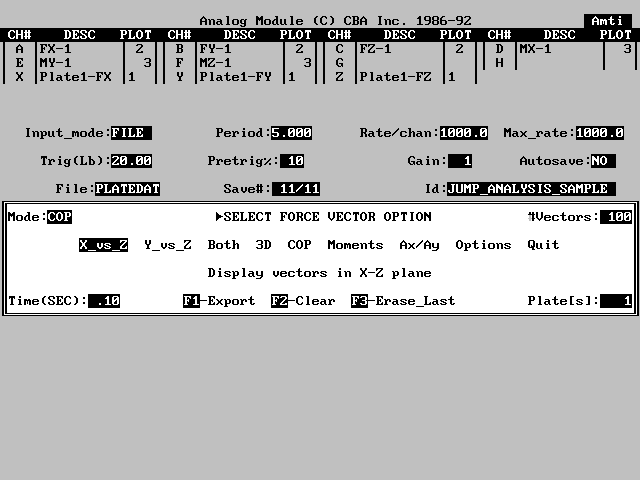
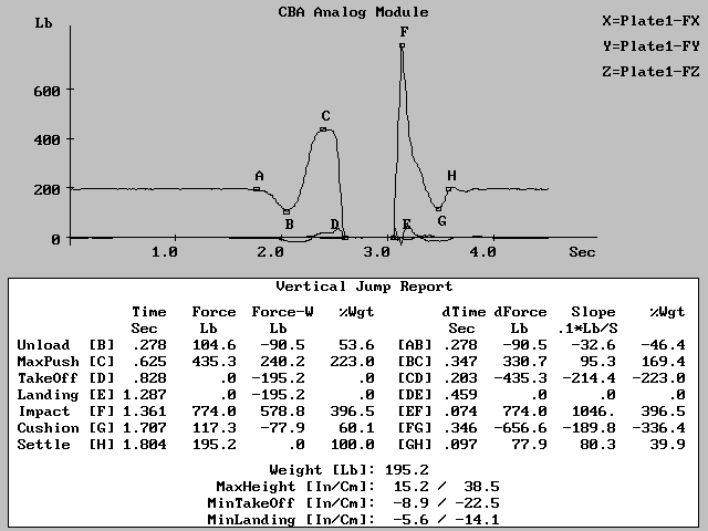
14.8.7.7 Jump Jump is selected to perform a vertical jump analysis using analog force plate data. for optimal results using this option several steps should be taken during data collection. First, the trigger level should be set to a negative value. this will allow data collection to be triggered from the keyboard. the plate should be zeroed when there is no weight on the plate. the subject should then step on the plate and remain motionless as the operator triggers the data collection with the keyboard. After approximately 1 to 2 seconds, the subject should jump and land back on the plate and remain still for approximately 5 seconds. The color graphics display shows the Vertical Jump Report Table below the graphed force platform data. eight points (labeled A through H) are labeled on the z direction force graph and are used for the row labels in the table. Column labels include Time, Force, Force-Weight, %Weight, Time change between points, Force change between points and Slope (impulse). Weight and max height are also listed below the table. the display on the color monitor can be sent to the printer by pressing the Ctrl and Print Scrn keys simultaneously. 14.8.8 Options The Options item on the Analog Processing Menu is identical to the display option from the Main Analysis Menu. 14.9 ADVANCING TO THE NEXT ANALOG SAMPLE The display and analysis options on the Analog Data Processing Menu (Figure 14-8) have now been discussed. On final step remains to complete the normal flow of analog processing; advancing to the next analog sample. When the processing of the current sample is complete, Quit is selected on the analog Processing Menu. Before returning to the main menu to allow additional sampling, the program displays a new menu. The first two options, Clear and Save, control the status of the graphic display following the next analog input, while the third option, Abort is used to cancel this quit command and return to the processing of the current analog sample. this latter option is provided to prevent inadvertent data loss since the current sample is discarded when the program returns to the Main Analog Menu (Figure 14-1). Clear is selected when the graphic display is to be cleared prior to graphing the next analog sample. this is the normal mode of display and results in each sample being graphed separately. Save is selected when the current display is to be retained and the next analog sample is to be graphed as a new graph on the same display. this option allows consecutive analog samples to be compared graphically.
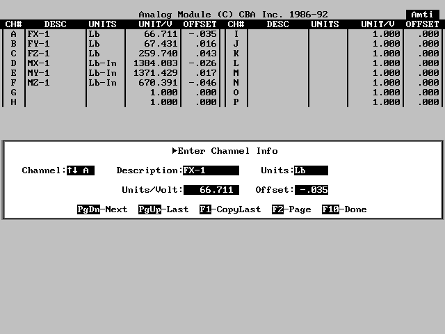
The analog to digital conversion hardware supplied with the analog module measures all analog input signals in volts. the normal input range is + 5 volts. Input should not exceed 5 volts for proper operation (this may require the addition of over voltage protection circuitry on some signal sources). the limit of resolution for signals in this voltage range is approximately 5 millivolts. All analog inputs being measured must use the same input voltage range. The inputs to the analog converter feature a high impedance (100M) and a low capacitance (dpf) to minimize the effect of the measurement process on the signal itself. Most types of analog signals can be directly measured by the analog hardware, however, certain signal sources such as strain gauges and transducers with frequency or current outputs will require external signal conditioners and/or conversion prior to measurement by the analog module. Once the analog signals are properly established, they are connected to the converter module using standard BNC type connectors. Sources with different types of connectors will require adapters that are readily available. signals should be connected to consecutive channels starting with channel A, then channel B, and so on. If channels are skipped for any reason, the input to that channel must be connected to ground. Floating or unterminated input channels may result in inaccurate data measurements. The individual input signals must mow be defined in the analog module. Select Options on the Main Analog Menu then select Channels on the Options Menu. A table of the possible analog channels will appear on the display. This is called the channel Definition Table. For each channel, this table contains:
Entry of an accurate conversion factor and offset for each channel is critical if measurements are to be reported correctly. for example, if force platform input is being measured, and it is desired to report results in pounds, the output of each force platform channel in pound/volts must be known and entered in the channel table. If the conversion factor is not known, use volts for Units and enter 1 for Units/V. Most laboratory measuring devices can be adjusted for a zero offset (i.e. zero volts of output signal equals zero measurement units). If analog signals do not have a zero volt offset, measure the actual offset corresponding to zero measurement units (this can be done using an analog channel with 1 unit/volt and a zero offset), and enter this value in the Channel Table. The measured signal will then be adjusted by this offset prior to being graphed or analyzed. Whenever a new data file is created in the analog module, the contents of the channel definition table, as well as the analog input parameters, are saved in that file. If there are several standard input configurations that will be used for sampling (e.g. force platform, EMG equipment, etc.) each channel and parameter configuration can be saved in a separate file. In this manner, one only needs to access an existing file in order to configure the analog module for a given type of data collection. In addition, the current configuration is saved on exit from the analog module and is restored when the module is run again. This completes the discussion of analog channel setup. In practice, one typically connects the input signals and then performs a series of trial measurements to establish signal levels, sampling times, and adjustment of signal sources to achieve proper calibration. A discussion of specific laboratory and clinical data measurement techniques is, however, beyond the scope of this manual. |
|
|
